






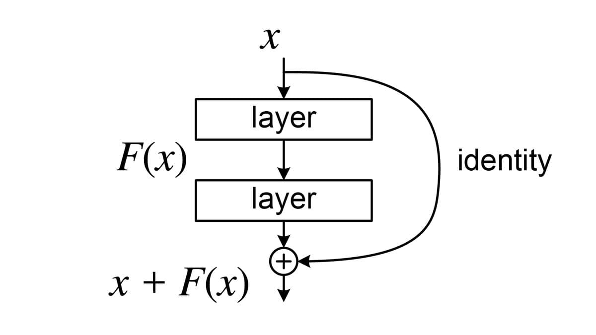
In December 2015, four researchers at Microsoft Research Asia posted a 12-page paper with one small idea in it. Take the input to a pair of layers, carry it around those layers untouched, and add it back to their output. That is the whole trick. It is one extra + in the code.
That paper, Deep Residual Learning for Image Recognition, is now the most cited research paper of the 21st century according to Nature's 2025 analysis. The idea it introduced, the residual connection, sits inside every large language model you use today. This guide explains what a residual connection is, the problem it solved, the four best explanations for why it works, and how a fix for image classifiers became the working memory of modern AI.
TL;DR: A residual connection adds a block's input back to its output:
y = F(x) + x. It fixed the 2015 degradation problem, let ResNet train 152 layers and win ImageNet at 3.57% top-5 error, and became the residual stream inside every transformer. The builder's lesson: add to a shared record, never overwrite it. Build with Taskade Genesis →
Quick answer: what is a residual connection? A residual connection (also called a skip connection) is a shortcut in a neural network that carries the input of a block around the block and adds it to the block's output. The block then learns only the difference it should make, which is called the residual. This makes very deep networks trainable, and it is used in ResNets, transformers, diffusion models and almost every deep model built since 2016.
In this guide: Quick facts · The 2015 depth wall · The paradox · The fix · The code · The results · The ResNet family · Why it works · The residual stream · Transformers and LLMs · Registers · What the story leaves out · Comparison · ResNets in 2026 · Timeline · For builders · FAQ
📌 Residual Connections at a Glance
A residual connection is a one-line change, y = F(x) + x, first published on December 10, 2015. It turned depth from a liability into an asset, and the paper that introduced it ranks first in Nature's 2025 analysis of the most cited papers of this century. The table below gives the facts most readers look for, each with its source.
| Fact | Value | Source |
|---|---|---|
| Paper | Deep Residual Learning for Image Recognition | arXiv 1512.03385 |
| Authors | Kaiming He, Xiangyu Zhang, Shaoqing Ren, Jian Sun (Microsoft Research Asia) | arXiv listing |
| Posted | December 10, 2015, 12 pages | arXiv listing |
| Venue | CVPR 2016, Best Paper Award | CVPR 2016 |
| Deepest ImageNet model | 152 layers, about 8 times deeper than VGG | Paper abstract |
| Headline result | 3.57% top-5 error (ensemble), 1st place ILSVRC 2015 | Paper, Table 5 |
| Citations | 103,756 to 254,074 across five databases (April 2025) | Nature |
| Citations today | 243,394 for the CVPR version on November 12, 2026 | OpenAlex |
| Rank | Most cited paper of the 21st century | Nature, April 2025 |
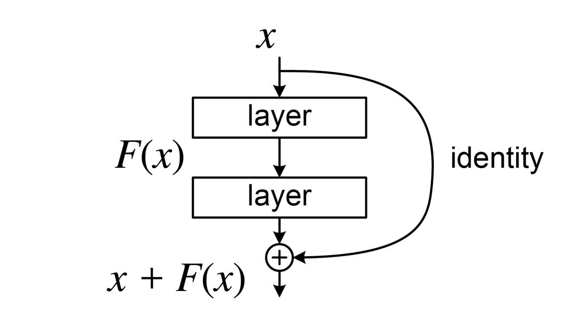
The whole idea in one picture. Two layers compute F(x), the identity path carries x around them, and the block outputs x + F(x). Diagram: Wikimedia Commons / LunarLullaby / CC BY-SA 4.0
One note on sources before we start. The best visual walk-through of this story is the Welch Labs video The most cited paper of the century is a brilliant hack. We use its demonstrations in two places below and label them as the video's own experiments. The Nature citation counts and ranks are as reported by outlets that reproduced Nature's table. The other numbers come from the original papers and the sources linked beside them.
🧱 What Was the Depth Wall of 2015?
The depth wall was the point, somewhere past 20 layers, where adding more layers to a neural network made it worse. From 2012 to 2014, the biggest jumps in ImageNet accuracy came with jumps in depth. In early 2015 that pattern broke, and nobody knew why.
The run-up is easy to chart. AlexNet won ImageNet in 2012 with eight learned layers and started the modern deep learning era. In 2014, Oxford's VGG reached 19 layers and Google's GoogLeNet reached 22. Both beat everything before them.
The error rate fell in step. The official ILSVRC summary paper records the winning top-5 classification error for 2012 through 2014, and the ResNet paper reports 2015.
The 2012 and 2013 figures are for entries trained only on the challenge data. AlexNet's better-known 15.3% used extra training data.
Then the trend stalled. In February 2015 the same Microsoft team published Delving Deep into Rectifiers, the paper that gave us He initialization. With the new initialization they could finally get a 30-layer network to train at all. With the older Xavier scheme, the paper reports, the 30-layer model "completely stalls". But the result was a letdown.
| Model (February 2015) | Top-1 error | Top-5 error |
|---|---|---|
| 14-layer network | 33.82% | 13.34% |
| 30-layer network | 38.56% | 16.59% |
The deeper model trained, and it lost. The authors wrote the puzzle down honestly: "This is perhaps because the method of increasing depth is not appropriate, or the recognition task is not enough complex."
Ten months later they named the effect. The ResNet paper calls it the degradation problem: "with the network depth increasing, accuracy gets saturated (which might be unsurprising) and then degrades rapidly." Its first figure shows a 56-layer plain network with higher error than a 20-layer one on CIFAR-10. The key detail is that the 56-layer network is worse on the training set too.
🚫 Why the Degradation Problem Is Not Overfitting
Overfitting means low training error and high test error. Degradation means high training error. A network that overfits has learned the training data too well. A network that degrades cannot even fit the training data, although it has more capacity than the shallow network that can.
The ResNet paper is direct about this: "Unexpectedly, such degradation is not caused by overfitting, and adding more layers to a suitably deep model leads to higher training error."
It also rules out the usual suspect. Most explainers say ResNet "solved the vanishing gradient problem". The paper itself says the opposite about its own experiments. The plain networks used batch normalization, the gradients had healthy norms, and the authors conclude: "We argue that this optimization difficulty is unlikely to be caused by vanishing gradients."
| Failure | What you see | Cause | Classic fix |
|---|---|---|---|
| Overfitting | Training error low, test error high | Model memorizes the training set | More data, regularization |
| Vanishing gradients | Early layers stop learning, loss stalls | Gradient shrinks at every layer | Better initialization, batch normalization |
| Degradation | Training error rises as depth grows | Optimizer cannot find a good deep solution | Residual connections |
So by late 2015 the field had a strange fact on its hands. Deeper networks were strictly more capable on paper, and worse in practice.
🧩 Why Could the Optimizer Not Find the Identity?
A deeper network can always match a shallower one by copying it and making the extra layers do nothing, yet gradient descent never found that solution. This is the paradox at the heart of the ResNet paper, and it is what made the degradation problem so confusing.
The argument is a construction. Take a trained 14-layer network. Build a 30-layer network by copying those 14 layers and adding 16 more that pass their input straight through. A layer that outputs exactly what it receives is called an identity mapping. The 30-layer network now gives the same answers as the 14-layer one, so its error can be no higher.
The paper states it plainly: "There exists a solution by construction to the deeper model: the added layers are identity mapping, and the other layers are copied from the learned shallower model." And then the punchline: "our current solvers on hand are unable to find solutions that are comparably good or better than the constructed solution."
Why is "do nothing" so hard to learn? A stack of layers with nonlinear activations has to arrange thousands of weights very precisely to reproduce its input. Starting from random weights, every layer scrambles the signal a little, and by the time 30 or 50 layers have each scrambled it, the feedback that reaches the early layers is too noisy to say what to change. The feedback is present. It is not usable.
The Welch Labs video shows this with a demonstration worth watching. It sweeps a single weight in the last layer of a small network and plots the model's confidence in the right answer. The curve is smooth. It repeats the sweep for a weight in the middle, then for a weight in the first layer, and the curve gets more and more jagged. The further a weight sits from the output, the more later layers distort its effect.
This is the same learning signal that powers all of how large language models work: the gradient, computed by backpropagation, tells each weight which way to move. If the gradient for early layers is noise, depth cannot help. The history of that signal goes back to the Widrow-Hoff rule of 1959.
➕ How Does a Residual Connection Work?
A residual connection takes the input to a block, routes it around the block unchanged, and adds it to the block's output: y = F(x) + x. The layers inside the block no longer learn the full transformation. They learn only F(x), the residual, which is the change to apply to the input.
The reasoning in the paper is short. If the ideal behavior of a block is to do nothing, a plain block must learn an exact identity through nonlinear layers, which is hard. A residual block only has to push its weights toward zero, which is easy. In the authors' words: "if an identity mapping were optimal, it would be easier to push the residual to zero than to fit an identity mapping by a stack of nonlinear layers."
In other words, the identity is no longer something the network must discover. It is wired in.
          PLAIN BLOCK                        RESIDUAL BLOCK

             x                                   x
             |                                   |-----------------+
        +---------+                         +---------+            |
        |  layer  |                         |  layer  |            |
        +---------+                         +---------+            |  identity
             |                                   |                 |  shortcut
        +---------+                         +---------+            |
        |  layer  |                         |  layer  |            |
        +---------+                         +---------+            |
             |                                   |                 |
             v                                  (+)<---------------+
          y = H(x)                               |
                                                 v
   The layers must learn                    y = F(x) + x
   the whole mapping H.               The layers learn only the
                                      change F. Doing nothing
                                      means F = 0.
The same pair, drawn as a flow:
Three practical details matter.
- The shortcut costs nothing. An identity shortcut adds no parameters and almost no computation. The paper notes that its ResNets "have no extra parameter compared to their plain counterparts".
- Shapes must match. You can only add two tensors of the same shape. When a block changes the number of channels or halves the resolution, the shortcut has to change shape too. The paper tests two ways: pad the extra channels with zeros, which adds no parameters and is what its 18 and 34-layer comparison uses, or apply a 1x1 convolution with stride 2 (a projection), which the deeper models use. It finds identity shortcuts are enough everywhere else.
- The block needs at least two layers. With a single layer,
y = Wx + xis just another linear layer, and the authors report they "have not observed advantages" from it.
🔀 Residual Connection vs Skip Connection: Is There a Difference?
A skip connection is the general term for any path that bypasses layers, and a residual connection is the specific kind that adds the unchanged input back. Most people use the two names for the same thing, and in a ResNet they are the same thing.
| Type | How the skipped signal is merged | Example |
|---|---|---|
| Residual (identity) | Added, unchanged | ResNet, transformers |
| Projection | Added, after a 1x1 convolution | ResNet downsampling blocks |
| Gated | Mixed by a learned gate | Highway Networks, LSTM |
| Dense | Concatenated, not added | DenseNet |
| Long skip | Carried across an encoder and decoder | U-Net style models |
💻 What Does a Residual Block Look Like in Code?
In PyTorch, a residual connection is the expression out + x on the last line of the block's forward pass. Everything else is an ordinary pair of convolutions with batch normalization. This is the basic block used in ResNet-18 and ResNet-34.
Python
import torch.nn as nn

class BasicBlock(nn.Module):
    """Two 3x3 convolutions with an identity shortcut (ResNet-18 and ResNet-34)."""

    def __init__(self, channels):
        super().__init__()
        self.conv1 = nn.Conv2d(channels, channels, 3, padding=1, bias=False)
        self.bn1 = nn.BatchNorm2d(channels)
        self.conv2 = nn.Conv2d(channels, channels, 3, padding=1, bias=False)
        self.bn2 = nn.BatchNorm2d(channels)
        self.relu = nn.ReLU(inplace=True)

    def forward(self, x):
        out = self.relu(self.bn1(self.conv1(x)))
        out = self.bn2(self.conv2(out))
        return self.relu(out + x)  # the residual connection
Delete + x and you have a plain network. That one term is the difference between a 34-layer model that degrades and one that does not.
🍾 What Is a Bottleneck Block?
A bottleneck block is a residual block with three convolutions (1x1, 3x3, 1x1) that squeezes the channels before the expensive 3x3 step and restores them after. ResNet-50, ResNet-101 and ResNet-152 use it to stay affordable at depth. The paper's example takes a 256-channel input down to 64 channels and back.
Python
class Bottleneck(nn.Module):
    """1x1 reduce, 3x3, 1x1 restore, with an identity shortcut (ResNet-50/101/152)."""

    def __init__(self, channels=256, width=64):
        super().__init__()
        self.reduce = nn.Conv2d(channels, width, 1, bias=False)
        self.bn1 = nn.BatchNorm2d(width)
        self.conv = nn.Conv2d(width, width, 3, padding=1, bias=False)
        self.bn2 = nn.BatchNorm2d(width)
        self.restore = nn.Conv2d(width, channels, 1, bias=False)
        self.bn3 = nn.BatchNorm2d(channels)
        self.relu = nn.ReLU(inplace=True)

    def forward(self, x):
        out = self.relu(self.bn1(self.reduce(x)))
        out = self.relu(self.bn2(self.conv(out)))
        out = self.bn3(self.restore(out))
        return self.relu(out + x)  # same shortcut, deeper function
The payoff shows up in the cost. The paper reports that its 152-layer ResNet needs 11.3 billion FLOPs, which is still less than the 19-layer VGG at 19.6 billion.
🏆 What Did ResNet Achieve?
ResNet removed the degradation problem in a controlled test, then won five tracks of the 2015 ImageNet and COCO competitions. The controlled test is the more important result, because it isolates the effect of the shortcut. Same depth, same parameters, same training, one + added.
The paper trained four networks on ImageNet: 18 and 34 layers, each with and without shortcuts.
| Depth | Plain network | ResNet | What changed |
|---|---|---|---|
| 18 layers | 27.94% | 27.88% | Almost nothing, but ResNet converges faster |
| 34 layers | 28.54% | 25.03% | Plain got worse with depth, ResNet got better |
Without shortcuts, going from 18 to 34 layers raised the error. With shortcuts, the same step lowered it by about 2.8 points, and the 34-layer residual network beat the 34-layer plain network by about 3.5 points. Depth was an asset again.
With that settled, the team scaled up. A single 152-layer ResNet reached 4.49% top-5 validation error, which the paper notes "outperforms all previous ensemble results". An ensemble of six models reached 3.57% top-5 error on the test set and won first place in ILSVRC 2015 classification. The abstract lists the rest of the sweep: first place in ImageNet detection, ImageNet localization, COCO detection and COCO segmentation, with a 28% relative improvement on COCO object detection from the deeper features alone.
Presenting the work at CVPR 2016, Kaiming He was dry about it. Welch Labs includes the clip: after showing the eight layers of AlexNet and the roughly 20 layers of VGG and GoogLeNet, he puts up a 152-layer ResNet and says, "it is not too special, it is just a lot of layers."
🎬 The Demonstration: 74 Layers With and Without Skips
Welch Labs re-runs the story on a small scale, and the numbers make the effect easy to feel. These are the video's own experiments, not results from the ResNet paper, and each row was trained for a different number of steps.
| Network in the Welch Labs demo | ImageNet accuracy reported in the video |
|---|---|
| 8 layers, plain | 44.1% |
| 14 layers, plain | 56.7% |
| 26 layers, plain | 63.6% |
| 74 layers, plain | 38.9% |
| 74 layers, with skip connections | 72.6% |
The 74-layer plain network does worse than the 8-layer one. Add skip connections, retrain, and it becomes the best model in the set. Source: Welch Labs.
🗂️ What Are ResNet-18, 34, 50, 101 and 152?
The ResNet family is five standard depths of the same design, named by their count of weighted layers. ResNet-18 and ResNet-34 stack basic blocks. ResNet-50, 101 and 152 stack bottleneck blocks. All five share the same four-stage layout and differ only in how many blocks each stage holds.
| Model | Block and stage layout | Parameters | FLOPs | Top-1 / top-5 accuracy |
|---|---|---|---|---|
| ResNet-18 | Basic, 2-2-2-2 | 11.7M | 1.8B | 69.76% / 89.08% |
| ResNet-34 | Basic, 3-4-6-3 | 21.8M | 3.6B | 73.31% / 91.42% |
| ResNet-50 | Bottleneck, 3-4-6-3 | 25.6M | 3.8B | 76.13% / 92.86% |
| ResNet-101 | Bottleneck, 3-4-23-3 | 44.5M | 7.6B | 77.37% / 93.55% |
| ResNet-152 | Bottleneck, 3-8-36-3 | 60.2M | 11.3B | 78.31% / 94.05% |
Sources: stage layouts and FLOPs from Table 1 of the ResNet paper. Parameters and single-crop ImageNet accuracy from the torchvision model documentation for the original IMAGENET1K_V1 weights.
Two things in this table are worth a second look.
- ResNet-50 is the sweet spot. It has almost the same compute as ResNet-34 (3.8 billion against 3.6 billion FLOPs) and clearly better accuracy, because the bottleneck block buys depth cheaply. That is why "ResNet-50" became the default baseline of computer vision.
- The same architecture got better with better training. torchvision also ships
IMAGENET1K_V2weights for ResNet-50 at 80.86% top-1, with no change to the network. The 2021 paper ResNet strikes back reports 80.4% for a vanilla ResNet-50 with a modern training recipe.
How does a number like 50 come about? Count the layers with weights: one opening convolution, 16 bottleneck blocks with three convolutions each (48), and one final fully connected layer. That makes 50.
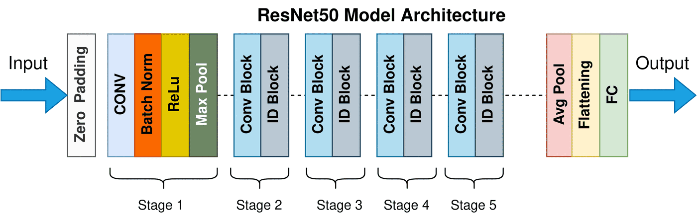
ResNet-50 from input to output: one stem, four stages of residual blocks, one classifier. Diagram: Wikimedia Commons / Gorlapraveen123 / CC BY-SA 4.0
🔬 Why Do Residual Connections Work?
Residual connections work for at least four reasons that researchers have tested: gradients get a direct path, gradients stay correlated, the network acts like many short paths, and the loss surface becomes smooth. The original paper showed that the idea works. It took three more years of papers to explain why, and the explanations overlap.
| Explanation | Claim | Evidence | Paper |
|---|---|---|---|
| Gradient highway | The identity path carries signals forward and backward without loss | Math, plus a 1,001-layer network at 4.62% CIFAR-10 error | He et al., 2016 |
| Shattered gradients | Plain-network gradients decorrelate with depth and look like white noise | Analysis and experiments on gradient correlation | Balduzzi et al., 2017 |
| Many short paths | A ResNet behaves like a collection of shallower networks | Layers can be deleted or reordered at test time | Veit et al., 2016 |
| Loss landscape | Skip connections keep the loss surface from turning chaotic | Visualizations of the same network with and without skips | Li et al., 2018 |
1. The Gradient Highway
The identity path gives every layer a direct line to the loss. Three months after ResNet, the same four authors published Identity Mappings in Deep Residual Networks. They showed that when the shortcut is a clean identity, the signal can travel from any block to any other block directly, in both directions. They then tested what happens when the shortcut is not clean (scaled, gated, or passed through a convolution) and found each change made training harder.
The paper also moved the normalization and activation to the front of each block, a design called pre-activation or ResNet v2. With it, a 1,001-layer network reached 4.62% error on CIFAR-10. Modern transformers use the same pre-normalization layout.
2. Gradients That Do Not Shatter
In a deep plain network, the gradient for one input tells you almost nothing about the gradient for a nearby input. The 2017 paper The Shattered Gradients Problem, subtitled "If resnets are the answer, then what is the question?", measured this. In its words, the correlation between gradients in standard feedforward networks "decays exponentially with depth resulting in gradients that resemble white noise", while with skip connections the gradients are "far more resistant to shattering, decaying sublinearly".
This is a strong candidate for the degradation puzzle. Gradients in deep plain networks do not have to vanish to become useless. They can be present and close to noise. One caution from the authors: the analysis applies at initialization, and how shattering affects training later is, in their words, "an important open problem".
3. Many Short Paths Instead of One Long One
A residual network is less like one deep pipeline and more like a huge collection of paths of different lengths. In May 2016, Andreas Veit, Michael Wilber and Serge Belongie at Cornell published Residual Networks Behave Like Ensembles of Relatively Shallow Networks.
At every block, a signal can go through the block or around it. With n blocks there are 2^n routes from input to output. The Cornell team studied a 110-layer ResNet with 54 blocks and found three things.
- You can delete layers. Removing a single block at test time barely changed the error, with a modest effect for the blocks that halve the resolution. In VGG, the paper reports, deleting any one layer drops performance to chance.
- You can shuffle layers. Reordering blocks degraded the error smoothly, not suddenly.
- Short paths do the work. Almost all of the gradient during training came from paths 5 to 17 blocks long, which the paper describes as 10 to 34 layers deep. Those paths are only 0.45% of all paths through the network.
Three blocks give eight paths. Fifty-four blocks give 2^54. Delete one block and half the paths remain, which is why the network shrugs it off.
4. A Smoother Loss Landscape
Skip connections turn a chaotic loss surface into a smooth one that gradient descent can walk down. In Visualizing the Loss Landscape of Neural Nets, Hao Li and colleagues plotted the loss of a 56-layer network along two random directions in weight space, once with skip connections and once without. Without skips, the surface is a field of spikes and pits. With skips, it is a smooth bowl. The paper concludes that skip connections "promote flat minimizers and prevent the transition to chaotic behavior".
The Welch Labs video reproduces this picture for its own 74-layer network, and it is the most convincing 30 seconds in the film. Loss landscapes also show up in research on grokking, where a network suddenly moves from memorizing to understanding.
These four explanations are views of one fact. A clean additive path keeps the learning signal intact across depth.
🌊 What Is the Residual Stream?
The residual stream is the running sum that flows from the input of a residual network to its output, with every block reading from it and adding to it. The term comes from interpretability research on transformers, but the picture applies to any network built from residual connections. It changes how you think a deep network computes.
In 2015 the standard mental model was a hierarchy. Layer one finds edges, layer two combines edges into corners, later layers find faces. Each layer builds on the one before it, so every layer is a critical link in a chain. The Cornell layer-deletion result did not fit that model. If every layer were a critical link, deleting one would break the chain.
Redraw the network and the result makes sense. Straighten all the shortcuts into one horizontal line, and draw each block as a side branch that reads from the line and writes back to it.
  x -----------+---------------+---------------+-----------> output
               |               |               |
            +--v--+         +--v--+         +--v--+
            |  F  |         |  G  |         |  H  |
            +--+--+         +--+--+         +--+--+
               |               |               |
              (+)             (+)             (+)

  after block F:   x + F
  after block G:   x + F + G
  after block H:   x + F + G + H        <- the final output

  Delete G and the output is  x + F + H.  The stream survives.
Nothing about the network has changed. It is the same wiring, drawn differently. But the new drawing shows something the old one hid: there is an unbroken channel from input to output, and each block makes an edit to it.
| Hierarchy view (before 2016) | Residual stream view (after) | |
|---|---|---|
| What a layer does | Transforms the previous layer's output | Reads a shared stream and adds an update |
| Where information lives | Passed on only through the latest layer's output | In the stream, visible to every later layer |
| Delete one layer | Chain breaks | One update is missing, the rest remain |
| Final output | Result of the last layer | Input plus the sum of all updates |
Both views hold at once. Klaus Greff, Rupesh Srivastava and Juergen Schmidhuber argued in Highway and Residual Networks learn Unrolled Iterative Estimation that groups of blocks refine the same level of representation step by step, while the network as a whole still moves from simple features to abstract ones.
🤖 How Do Transformers and LLMs Use Residual Connections?
Every transformer layer wraps its attention step and its MLP step in a residual connection, so the residual stream is the spine of every large language model. The 2017 paper Attention Is All You Need says so in one line: "We employ a residual connection around each of the two sub-layers, followed by layer normalization." It cites the ResNet paper for the idea.
In code, one layer of a modern language model is two additions.
Python
# One transformer layer, pre-norm layout
x = x + attention(norm1(x))  # tokens exchange information
x = x + mlp(norm2(x))        # each token processes what it gathered
Stack that a few dozen times and you have the core of the models behind ChatGPT, Claude and Gemini. The attention mechanism gets the headlines, but attention only computes the update. The residual connection is what carries the result forward.
The name "residual stream" was popularized by Anthropic's 2021 paper A Mathematical Framework for Transformer Circuits, which describes the model this way: "All components of a transformer (the token embedding, attention heads, MLP layers, and unembedding) communicate with each other by reading and writing to different subspaces of the residual stream." The paper calls the stream "a communication channel, since it doesn't do any processing itself and all layers communicate through it."
This is why the residual stream is the main object of study in mechanistic interpretability. When researchers find a "circuit" inside a model, they are tracing a path of reads and writes through the stream. When they train sparse autoencoders to find features, they are usually decomposing the stream at one layer. The stream is where a model's internal representations live.
The idea is still being refined. Moonshot's Kimi team published Attention Residuals in March 2026, which replaces the fixed sum with attention over earlier layer outputs. Our Kimi history covers how that fits into their models.
🧠 What Are Register Tokens, and Why Does the Stream Act Like Working Memory?
Register tokens are extra learned slots added to a vision transformer's input so the model has a dedicated place to keep global information. They were added to vision transformers after researchers caught a model building its own storage out of spare parts. The paper credits an earlier idea, Memory Transformers (Burtsev et al., 2020). The finding is strong evidence that a model uses the positions in its residual stream as working memory: when no position is set aside for global notes, it takes over positions that carry little information.
In September 2023, Timothée Darcet, Maxime Oquab, Julien Mairal and Piotr Bojanowski (Meta and Inria) published Vision Transformers Need Registers. They were studying DINOv2, a computer vision model whose largest version (ViT-g) has 40 layers. A vision transformer cuts an image into patches, and each patch gets its own position in the residual stream.
They noticed something odd in the largest model. Partway through the network, around layer 15, a few patch positions developed huge values. The paper measures about 2.37% of tokens with a norm above its outlier threshold. And those positions were not on the subject of the photo. They sat on background areas with little information: walls, sky, floor.
Their hypothesis, quoted from the paper: the model learns "to recognize patches containing little useful information, and recycle the corresponding tokens to aggregate global image information while discarding spatial information." In plain terms, the model needed scratch space for facts about the whole image, had none, and took over the patches it judged least useful.
They tested it with a linear probe: train a simple classifier on a single token and see what it knows.
| Dataset | Normal patch token | High-norm patch token | Class token |
|---|---|---|---|
| ImageNet-1k | 65.8% | 69.0% | 86.0% |
| Aircraft | 17.1% | 79.1% | 87.3% |
| CUB birds | 18.6% | 84.9% | 91.3% |
| Cars | 10.8% | 85.2% | 91.5% |
Source: Table 1 of Vision Transformers Need Registers. A normal patch knows about its own patch. A high-norm patch knows about the whole picture. The same tokens scored lower than normal patches on local tasks, such as predicting their own position, which fits the story: the local information was overwritten.
The fix was to give the model what it was improvising. The team added a few new tokens to the input that correspond to no image patch, start from learned values, and are thrown away at the output. They called them registers, a name that echoes the small storage slots in a CPU. Most experiments in the paper use four.
With registers in place, the high-norm artifacts vanished from the patch grid. The model moved its global bookkeeping into the slots it was given. The paper won an Outstanding Paper Award at ICLR 2024.
Language models show the same habit. One day after the registers paper, a separate team posted Efficient Streaming Language Models with Attention Sinks, which found that language models pile attention onto the first token regardless of its content, and proposed a dedicated placeholder token for that job. A 2024 paper, Massive Activations in Large Language Models, found a handful of enormous activations that act like fixed bias terms.
The pattern across all three is the one to remember. A model with no assigned place for shared state will make one, usually out of the least meaningful position it can find. Giving it a proper place works better.
🕵️ What Does the Popular ResNet Story Leave Out?
The usual telling skips three things: the shortcut idea had clear ancestors, the 1,202-layer network was not a win, and the version most people use today is a later refinement. None of this takes away from the paper. It makes the history more accurate.
| The popular version | The fuller picture | Source |
|---|---|---|
| ResNet invented the shortcut | Highway Networks trained very deep nets with gated shortcuts seven months earlier, building on the LSTM of 1997 | Srivastava et al., May 2015 |
| ResNet trained 1,202 layers, so deeper is better | The 1,202-layer net scored 7.93% error, worse than the 110-layer net at 6.43% | ResNet paper, Table 6 |
| ResNet fixed vanishing gradients | The paper says the difficulty is unlikely to be vanishing gradients | ResNet paper, Section 4.1 |
| The 2015 block is the final design | Pre-activation (v2) blocks arrived in March 2016 and are closer to what transformers use | He et al., 2016 |
Highway Networks came first. Rupesh Srivastava, Klaus Greff and Juergen Schmidhuber posted Highway Networks on May 3, 2015. A highway layer has a learned gate that decides how much of the input to carry through unchanged, an idea borrowed from the long short-term memory (LSTM) network that Sepp Hochreiter and Schmidhuber published in 1997. The highway paper reports optimizing networks up to 900 layers deep. The ResNet paper cites it and draws the line clearly: highway shortcuts are gated and have parameters, ResNet's are always open and have none. ResNet's contribution was the argument, backed by its results, that the shortcut should be a plain identity. Shortcut connections of various kinds appear in neural network research long before either paper, as Wikipedia's history of residual networks traces.
The 1,202-layer network lost. The paper trained it on CIFAR-10 to show that optimization no longer breaks at extreme depth. It worked in that sense. But its test error was worse than the 110-layer network's, and the authors say why: "We argue that this is because of overfitting." Residual connections make depth trainable. They do not make depth free.
The story also has a human scale. Kaiming He was at Microsoft Research Asia from 2011 to 2016, then at Facebook AI Research, and joined MIT in 2024. His homepage today lists him as a tenured associate professor at MIT and a part-time Distinguished Scientist at Google DeepMind. It also states the reach of the idea without exaggeration: residual connections are used in "Transformers (e.g., ChatGPT), AlphaGo Zero, AlphaFold, and virtually all GenAI models today".
⚖️ ResNet vs VGG vs DenseNet vs Transformer: What Is the Difference?
VGG has no shortcuts, ResNet adds the input back, DenseNet concatenates every earlier output, and the transformer uses ResNet's additive shortcut around attention and MLP layers. All four are deep stacks. They differ in how information from earlier layers reaches later ones.
| Architecture | Year | How layers connect | Typical depth | Role today |
|---|---|---|---|---|
| VGG | 2014 | Plain chain, no shortcuts | 16 to 19 layers | Historical, some feature extraction |
| ResNet | 2015 | Add input to output | 18 to 152 layers | Standard vision baseline and backbone |
| DenseNet | 2016 | Concatenate all earlier outputs | 121 to 201 layers | Niche, strong feature reuse |
| Transformer | 2017 | Add input to output, around attention and MLP | Dozens of layers | Language models, vision transformers |
The VGG comparison shows how much the shortcut buys. The VGG paper lists 144 million parameters for its 19-layer model. ResNet-152 is eight times deeper with about 60 million parameters and, per the ResNet paper, fewer FLOPs.
DenseNet took the opposite route to ResNet. It keeps every earlier output and concatenates them, so nothing is ever merged by addition. That preserves information at the cost of memory.
The transformer is the most important descendant. It dropped convolutions and kept the shortcut. If you want the short version of the last decade of architecture research: the layers inside the block changed completely, and the + x around the block did not change at all.
📅 Are ResNets Still Used in 2026?
Yes. ResNets remain the default baseline in computer vision and a common backbone in production systems, even though newer models score higher. The design is simple, well understood, cheap to run and supported everywhere, which counts for a lot outside of leaderboards.
A live signal: the timm library on Hugging Face is the main open source collection of vision models. On November 12, 2026, sorted by downloads in the past month, two of its top four models were ResNets.
| timm model | Downloads in the past month (Nov 12, 2026) |
|---|---|
| mobilenetv3_small_100 | 11.0 million |
| tf_efficientnetv2_s | 3.6 million |
| resnet18.a1_in1k | 2.0 million |
| resnet50.a1_in1k | 1.7 million |
There are three reasons the family has lasted.
- Training recipes caught up. ResNet strikes back showed in 2021 that a plain ResNet-50 reaches 80.4% top-1 on ImageNet with modern training, far above its original score.
- Its successors are still ResNets at heart. ConvNeXt, titled "A ConvNet for the 2020s", starts from a standard ResNet and modernizes it step by step. ResNeXt, Wide ResNet and vision transformers all keep the residual connection.
- It is the reference point. When a paper proposes a new vision method, a ResNet-50 run is usually how readers judge it.
The architecture named ResNet may fade over time. The residual connection will not, because almost every very deep network in use today has some form of it. Researchers have trained deep networks without shortcuts by careful initialization, including in the shattered gradients paper itself, but those methods have not replaced it in practice.
🗓️ Residual Connections Timeline: 1997 to 2026
The road from gated memory cells to the residual stream took about 25 years, with the decisive step in December 2015. Each entry below links to its primary source.
| Date | Milestone | Why it matters |
|---|---|---|
| 1997 | LSTM (Hochreiter and Schmidhuber) | The constant error carousel, a self-connection with a weight of 1, lets error signals flow across many time steps |
| 2012 | AlexNet, 8 layers | Starts the deep learning era on GPUs |
| Sep 2014 | VGG (19 layers) and GoogLeNet (22 layers) | Depth drives accuracy |
| Feb 2015 | He initialization and batch normalization | 30 layers can train, but accuracy drops |
| May 2015 | Highway Networks | Gated shortcuts train very deep networks |
| Dec 10, 2015 | ResNet | Identity shortcuts, 152 layers, 3.57% top-5 error |
| Mar 2016 | Identity Mappings (ResNet v2) | Pre-activation blocks, 1,001 layers |
| May 2016 | Ensembles of shallow networks | Layers can be deleted and shuffled |
| Jun 2016 | ResNet wins the CVPR Best Paper Award | Recognition from the field |
| Feb 2017 | Shattered gradients | Shows that gradients in deep plain networks look like noise at initialization |
| Jun 2017 | Attention Is All You Need | Residual connections move into the transformer |
| Dec 2017 | Loss landscape visualization | Shows skips smooth the loss surface |
| Dec 2021 | Transformer Circuits framework | The name "residual stream" enters wide use |
| Sep 2023 | Vision Transformers Need Registers | A model is caught using spare token positions as working memory |
| Apr 2025 | Nature citation analysis | ResNet ranked the most cited paper of the century |
| Mar 2026 | Attention Residuals | Learned weights over the residual sum |
For the wider arc this sits inside, see our history of computing and the NVIDIA history, which covers the GPUs that made any of these experiments possible.
🛠️ What Do Residual Connections Teach People Who Build With AI?
Residual connections teach three design lessons that apply well beyond neural networks: build the default in, give shared state a home, and add to the record instead of replacing it. You do not need to train a model to use them.
Lesson 1: do not hope the system learns the safe default. Wire it in. Every layer in a 2015 network was capable of passing its input through. The optimizer did not find that behavior, so ResNet built it into the structure. The same applies to any system with a learning or generating component. If a behavior must always happen, make it part of the plumbing.
Lesson 2: if you give a system no place for shared state, it will improvise one. DINOv2 stored its global notes in background patches because it had nowhere else. Teams do the same thing with status updates buried in chat threads, and AI agents do it when their only memory is a long conversation.
Lesson 3: add, never overwrite. In a residual network no block replaces the stream. Each one reads what is there and contributes an update. That is why you can remove a block and keep working, and why the early signal is still available at the end.
This is an analogy, and it is worth saying so plainly. A workspace is not a neural network, and nothing here is a claim about how any product's models are built. The parallel is in the design choice. A team of AI agents works better when the agents share a durable record that each one reads and adds to, in the same way that layers work better when they share a stream. Our guides to AI agent memory and the history of agent memory go into what that record should hold.
It is the idea behind how Taskade is organized. Projects hold the memory. AI agents read that memory and add to it. Automations execute and write the results back. When you build an app with Taskade Genesis, Taskade EVE can set up those three parts together, so the record exists from the first step and every later step builds on it. You can see working examples in the Taskade App Factory.
Related reading on how models work inside:
- What is mechanistic interpretability? for how researchers read the residual stream
- What is grokking in AI? for another case where a simple training effect changed the theory
- AI inference explained for what happens when a trained model answers you
- How AI data centers work for the hardware under all of it
- Cross-entropy explained for the loss function behind the landscapes above
- AI world models and reasoning models for where architectures are going next
- What is intelligence? for the bigger question
- Open source LLMs if you want to inspect a residual stream yourself
❓ Frequently Asked Questions
What is a residual connection?
A residual connection is a shortcut that adds the input of a group of layers to the output of those layers, so the block computes y = F(x) + x instead of y = F(x). The layers only have to learn the change to make to the input, called the residual. Kaiming He, Xiangyu Zhang, Shaoqing Ren and Jian Sun introduced the design in the ResNet paper in December 2015.
What is the difference between a residual connection and a skip connection?
A skip connection is any path that lets a signal bypass one or more layers. A residual connection is the most common kind: the skipped signal is the unchanged input, and it is merged back by addition. DenseNet uses skip connections that concatenate, and Highway Networks use skip connections with learned gates. In everyday use the two terms are often treated as the same thing.
What problem did ResNet solve?
ResNet solved the degradation problem. Before ResNet, adding layers to an already deep network made its training error go up. The ResNet paper shows a 56-layer plain network with higher training and test error than a 20-layer one on CIFAR-10. With residual connections, a 152-layer network trained well, and an ensemble reached 3.57% top-5 error on ImageNet to win ILSVRC 2015.
Is the degradation problem the same as the vanishing gradient problem?
No. The ResNet paper says the difficulty is unlikely to be caused by vanishing gradients, because its plain networks used batch normalization and showed healthy gradient norms. It is also not overfitting, because training error gets worse too. Later work described a related effect, the shattered gradients problem: at initialization, gradients in deep plain networks lose their correlation and look like white noise.
Why do residual connections work?
Research supports four linked explanations. The identity path gives gradients a direct route to early layers. Skip connections keep gradients correlated instead of shattered. A residual network behaves like a large collection of shorter paths, so no single layer is critical. And the loss surface becomes much smoother, so gradient descent can find a good solution.
What is a bottleneck block in ResNet-50?
A bottleneck block is a residual block with three convolutions: a 1x1 convolution that reduces the channels, a 3x3 convolution that works on the smaller tensor, and a 1x1 convolution that restores the channels. ResNet-50, ResNet-101 and ResNet-152 use bottleneck blocks so that very deep networks stay affordable. ResNet-18 and ResNet-34 use a basic block with two 3x3 convolutions.
What is the residual stream in a transformer?
The residual stream is the running sum that flows through a transformer from the token embedding to the output. Every attention layer and every MLP layer reads from the stream and adds its result back. Anthropic researchers popularized the name in 2021 in A Mathematical Framework for Transformer Circuits. It is the object that mechanistic interpretability research reads to understand a model.
Do large language models use residual connections?
Yes. The 2017 transformer paper puts a residual connection around every attention sub-layer and every feed-forward sub-layer, and modern large language models keep that design. Without it, a stack of dozens of transformer layers would be very hard to train. Our guide to how LLMs work covers the rest of the architecture.
What are register tokens?
Register tokens are extra learned tokens added to the input of a vision transformer to give the model a dedicated place for global information. A Meta and Inria team added them to vision transformers in 2023 after finding that DINOv2 stored whole-image information in a small share of background patches with very high norms. With registers, those artifacts disappear. The paper won an Outstanding Paper Award at ICLR 2024.
Is ResNet really the most cited paper of the 21st century?
Yes, by the best available ranking. In April 2025, Nature combined five citation databases and ranked Deep Residual Learning for Image Recognition first among papers published this century. As reported by outlets that reproduced Nature's table, the paper had between 103,756 and 254,074 citations depending on the database, Attention Is All You Need ranked seventh and the AlexNet paper eighth.
Are ResNets still used in 2026?
Yes. ResNets are still the standard baseline and a common backbone in computer vision. On November 12, 2026, two ResNet checkpoints were among the four most downloaded timm models on Hugging Face. Newer designs such as ConvNeXt and vision transformers reach higher accuracy, and all of them keep the residual connection.
Did Highway Networks come before ResNet?
Yes. Rupesh Srivastava, Klaus Greff and Juergen Schmidhuber posted Highway Networks on May 3, 2015, seven months before ResNet. A highway layer has a learned gate that decides how much input to carry through, an idea taken from the LSTM of 1997. ResNet removed the gate and made the shortcut a plain identity, and the ResNet paper cites Highway Networks as related work.
🚀 Build on a Record That Remembers
Max Planck thought his 1900 quantum hypothesis was a mathematical trick. Thirty years later it had rewritten physics. Welch Labs closes its film with that comparison, and it fits. A residual connection began as a fix for an optimization bug in image classifiers. It ended up changing what researchers think a deep network is: a shared stream that many small steps read and add to.
The same shape works for teams and their AI. Keep one durable record. Let every agent, teammate and automation read it and add to it. Do not make anyone start from zero.
That is what a Taskade workspace gives you: projects that remember, agents that think with that memory, and automations that act on it. Create your first app with Taskade Genesis and watch each step build on the last: ▲ Memory, ■ Intelligence, ● Execution.