





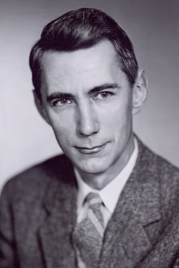
In 1951, Claude Shannon published a strange little experiment. He took a passage of English, showed a reader one letter at a time, and asked them to guess what came next. Correct guess, he wrote a dash. Wrong guess, he wrote down the true letter and moved on.
Of the 129 letters in his published sample, the guesser got 89 right. The page Shannon produced was far shorter than the original, and he argued it carried exactly the same information, because anyone with the same command of English could take that reduced page and reconstruct the original text from it. The correct guesses were free. Only the mistakes had to be written down.
That experiment is the whole idea behind a modern language model, worked out seventy years early with a pencil. And it points at something that sounds like a slogan but turns out to be a theorem: the better you can predict something, the smaller you can compress it. Prediction and compression are two views of one quantity, and the number that measures both is called cross-entropy.
TL;DR: Cross-entropy is the average number of bits wasted when you model data with the wrong probabilities. It is the loss function used to train every large language model, and because bits are literally units of file size, a model's training loss is its compression rate. Shannon proved the floor in 1948. Taskade Genesis applies the same principle: shared context means fewer bits to transmit.
What Is Cross-Entropy?
Cross-entropy is the average number of bits needed to encode data from one probability distribution when you are using a code optimized for a different distribution. Written formally, it is the sum of p times -log2(q), where p is how the world actually behaves and q is what your model believes. It hits its minimum only when q equals p.
That definition contains the entire reason it is the loss function of choice in machine learning. You cannot score well on cross-entropy by being lucky, by being vague, or by being confidently wrong. The only way down is to make your model's beliefs match reality.
Most explanations of cross-entropy stop at "it is a classification loss." That leaves out the more interesting half of the story, which is that the units are bits, the bits are real, and the number on your training dashboard is a measurement of how well your model could compress the internet.
Here is the chain this article walks, end to end:
Nobody gets to skip a link in that chain. So we will start at the beginning, with a robot on a moon.
Why Information Needs a Unit
Information is measured in bits, and the information content of an event is -log2(p), where p is the probability of that event. An event with a 1-in-8 chance carries 3 bits. A near-certain event carries almost none. The formula is not a convention chosen for convenience; it falls out of asking what perfect compression would have to look like.
To see why, take a deliberately small problem. You are sending movement instructions to a robot on a distant moon. There are four possible commands, and they are not equally likely.
| Instruction | Probability | Naive code | Better code | Bits used |
|---|---|---|---|---|
| Up | 1/2 | 00 |
0 |
1 |
| Down | 1/4 | 01 |
10 |
2 |
| Left | 1/8 | 10 |
110 |
3 |
| Right | 1/8 | 11 |
111 |
3 |
The naive scheme spends a flat 2 bits on every instruction. The better scheme spends 1 bit on the common one and 3 bits on the rare ones. Work out the weighted average and the second scheme costs 1.75 bits per instruction. It wins because it spends its bits where the uncertainty actually is.
Why the second code is decodable at all
Variable-length codes are easiest to decode when no codeword is a prefix of another one. This is called a prefix-free code, and it can be decoded instantly, symbol by symbol. Codes that break the rule can still be uniquely decodable, but only with delay, because the reader may have to look ahead before it can commit. The receiver reads bits until the sequence forms a complete codeword, commits it, and starts fresh, with no ambiguity and no separators needed.
Look at what each choice costs. Assigning the single bit 0 to Up consumes half of all possible codewords, because everything beginning with 0 is now off limits. Assigning 10 to Down eats a quarter. The two 3-bit codes eat an eighth each. Add them up and you get exactly 1.0, with nothing wasted.
Now notice the coincidence: the share of codeword space each instruction consumes is exactly its probability. One half, one quarter, one eighth, one eighth. That alignment is not luck. It is the seed of the whole theory.
The argument that pins the formula down
Here is the step that turns a coincidence into a definition. A perfect compressor must produce output indistinguishable from random noise, because any leftover pattern is a pattern you could have compressed away. Random noise means every bit is an independent coin flip.
So if a compressed message is n bits long, it is one of 2^n equally likely strings, which means the original message must have had probability 1/2^n. Take the logarithm of both sides and negate:
   message probability  =  2^-n
   take log2 of both sides
   log2(p)              =  -n
   negate
   n                    =  -log2(p)   bits to encode a message  =  -log2( probability of that message )
Read -log2(p) as "how many times do you cut the space of possibilities in half to get down to this one outcome." Rare things need many cuts. Common things need few.
This is why a weather forecast saying "sunny in the Sahara" tells you almost nothing, and one saying "snow in the Sahara" tells you a great deal. Information is surprise, measured in halvings.
Entropy: The Floor Nobody Can Beat
Entropy is the average information per symbol in a data source, calculated as the sum of p times -log2(p) across every possible symbol. It represents the theoretical minimum bits per symbol for lossless compression. For the robot above, entropy is exactly 1.75 bits, which is why the second code could not be improved.
Shannon proved two things about this number in 1948, and together they are called the source coding theorem (also known as the noiseless coding theorem):
- No encoding can ever do better than entropy, averaged over all messages.
- It is always possible to design an encoding that gets arbitrarily close to it.
That is an unusually strong pair of results. Entropy is not a rule of thumb. It is a wall, and you can always walk right up to it.
How the shape of a distribution changes its entropy
| Distribution over 4 symbols | Probabilities | Entropy | Reading |
|---|---|---|---|
| Uniform | 25 / 25 / 25 / 25 | 2.00 bits | Maximum uncertainty |
| Mildly skewed | 50 / 25 / 13 / 12 | 1.75 bits | The robot |
| Heavily skewed | 90 / 6 / 2 / 2 | 0.61 bits | Nearly predictable |
| Degenerate | 100 / 0 / 0 / 0 | 0.00 bits | No information at all |
The pattern is intuitive once you see it. Spread the probability evenly and every symbol is a genuine surprise, so entropy is high. Concentrate it on one outcome and there is almost nothing to tell anyone, so entropy collapses toward zero. A message you could have predicted costs nothing to send.
For the simplest possible case, a single biased coin, you can watch the whole curve:
Maximum at a fair coin, zero at either certainty. This curve reappears later in a way that matters.
Shannon's Experiment: Measuring English With a Human Brain
Shannon wanted the entropy of English, and he could not compute it. There is no formula for the probability distribution of a language. So in 1951 he published a paper that measured it by interrogating people instead, and the method is more interesting than the number.
His first instinct was pure data analysis. Count letter frequencies, then letter pairs, then triples, and extrapolate. This works for a while and then falls apart, because the interesting predictability in language lives in long context, and almost every long string of text appears zero times in any corpus you can assemble. You cannot get statistics on something you have never seen.

So he switched instruments. He gave people text with the next letter hidden and recorded how many guesses they needed to get it right, then converted guess counts into implied probabilities. The interviewee's brain was the model. He could not open it or write it down, but he could query it.
What the guessing games showed
Shannon worked with a 27-symbol alphabet, the 26 letters plus a space. These are the figures he published:
| Model of English | Context available | Bits per character |
|---|---|---|
| Raw 8-bit storage | none | 8.00 |
| Uniform over 27 symbols | none | 4.76 |
| Letter frequencies | none | 4.03 |
| Letter pairs, then triples | 1 to 2 characters | 3.32, then 3.10 |
| Word frequencies | previous word | 2.14 |
| Human guesser | 99 preceding letters | 0.6 to 1.3 |
The numbers fall off a cliff as context grows. That trend is the single most important fact in this article, because it is the same curve that governs how well a language model performs as its context window grows. More context means better prediction means fewer bits.
That final row is a bound rather than a point estimate. Shannon's own summary was that long-range effects up to 100 letters reduce the entropy to "something of the order of one bit per letter, with a corresponding redundancy of roughly 75%." Against plain 8-bit storage, that is roughly an 8 to 1 compression ratio sitting there for anyone who understands English well enough to claim it. He was careful to add that the redundancy may be higher still once structure spanning paragraphs and chapters is counted.
The part that matters most
Read that methodology again. Shannon could not measure the compressibility of language without borrowing an intelligence. He needed a system with a deep, working, non-writable model of English, and in 1951 the only such systems were people.
That is the first appearance of the thesis. Compression of a rich signal is not a mechanical operation you can perform with a clever algorithm alone. It requires a model of the thing being compressed, and the better the model understands, the better the compression. Shannon had to rent a brain. Seventy years later we build them.
Cross-Entropy: The Bill You Pay for a Wrong Model
Cross-entropy is what happens when the model you compress with does not match the world you compress. It answers a practical question: if I optimized my code for distribution q and reality turns out to follow distribution p, how many bits per symbol will I actually spend?
Go back to the robot. Suppose the mission changes and the command frequencies rotate: Up and Down become rare at 1/8 each, Left becomes 1/4, and Right dominates at 1/2. Your encoder is already built and hard-coded for the old distribution. What does that cost?
  old code (optimized for the OLD mission):
    Up = 0 (1 bit)   Down = 10 (2 bits)   Left = 110 (3 bits)   Right = 111 (3 bits)  new reality:
Up 1/8           Down 1/8             Left 1/4              Right 1/2
  bill = (1/8 x 1) + (1/8 x 2) + (1/4 x 3) + (1/2 x 3)
= 0.125 + 0.25 + 0.75 + 1.5
= 2.625 bits per instruction
  entropy of the new mission = 1.75 bits    <-- what a correct model would pay
cross-entropy              = 2.625 bits   <-- what the stale model pays
wasted (KL divergence)     = 0.875 bits   <-- pure penalty for being wrong
That 2.625 is the cross-entropy of the old model relative to the new reality. The formula generalizes directly:
   H(P, Q)  =  sum over i of   p_i  x  ( -log2( q_i ) )
                               ^^^          ^^^
                       reality's weights   model's bit-lengths
Reality decides how often each symbol shows up. Your model decides how many bits each one costs. Cross-entropy multiplies them together.
Order matters, and that tells you something
Cross-entropy is not symmetric. Swapping the model and reality gives a different answer, and the asymmetry is the most practically useful thing about it.
| Model believes (Q) | Reality is (P) | Entropy of P (the floor) | Cross-entropy | Penalty |
|---|---|---|---|---|
| 50 / 50 | 90 / 10 | 0.47 bit | 1.00 bit | 0.53 bits, wasteful |
| 90 / 10 | 50 / 50 | 1.00 bit | 1.74 bits | 0.74 bits, severe |
Read the two rows carefully, because this is the whole intuition for why cross-entropy is a good loss function.
Note that the floor is always the entropy of reality, never the entropy of your model. That is why neither row escapes a penalty: the model is wrong in both, so it pays in both.
In the first row the model is uncertain and reality is predictable. The model spends 1 bit on everything when 0.47 would do, which is wasteful but survivable. In the second row the model is confident and wrong. It bet almost everything on one outcome, so when the other one keeps showing up it pays over 3 bits every time, and the average balloons.
Confident and wrong is the expensive failure. Uncertain is cheap. A loss function with that property teaches a model to be honestly calibrated instead of boldly guessing, which is exactly what you want.
The one property to remember
Fix reality at P and let the model Q vary. Cross-entropy traces a bowl. It has a single minimum, that minimum sits exactly where Q = P, and the value at the bottom is the entropy of P.
Three consequences follow immediately, and they are why every deep learning framework ships this function:
- It cannot be gamed. The only route to a lower score is a better model.
- It has a known floor. You can tell how much improvement is even theoretically left.
- It punishes false confidence. The negative logarithm grows without bound as the predicted probability of the true answer approaches zero.
Cross-Entropy vs KL Divergence vs Log Loss
These three terms describe closely related quantities and are frequently confused. Cross-entropy is the total bits spent. KL divergence is cross-entropy minus entropy, isolating only the waste. Log loss is simply another name for cross-entropy, inherited from the statistics literature rather than the information theory one.
| Term | Formula | What it measures | When you see it |
|---|---|---|---|
| Entropy | sum p x -log2(p) |
Irreducible floor | Theory, compression limits |
| Cross-entropy | sum p x -log2(q) |
Total bits paid | Training loss, LLM pre-training |
| KL divergence | H(P,Q) - H(P) |
Waste from a wrong model | Distillation, regularization, RLHF |
| Log loss | Same as cross-entropy | Total bits paid | Binary classification, statistics |
| Perplexity | 2^(cross-entropy) |
Effective branching factor | Language model evaluation |
The practical question people actually have is why frameworks minimize cross-entropy rather than KL divergence, given that KL is the quantity you philosophically care about. The answer is that they differ by the entropy of the data, which is a constant you cannot change. Minimizing either one produces the identical optimal model, and cross-entropy is the one you can compute without knowing the true distribution.
Perplexity deserves a note because it is the number most often quoted in language model papers. It is just cross-entropy exponentiated, which converts bits into "effective number of equally likely choices." A perplexity of 8 means the model is as uncertain as if it were picking uniformly among 8 options. Lower is better, and it carries exactly the same information as the loss.
The Duality: Why Training Loss Is a Compression Rate
Pre-training a language model minimizes cross-entropy over the training corpus. Because cross-entropy is measured in bits, and bits are the unit of file size, the training loss is not merely analogous to a compression rate. It is one. A model with a loss of 2 bits per token could compress its training data to 2 bits per token.
Assemble the pieces already established:
- A perfect code spends
-log2(p)bits on an event. - The information of a whole message is the sum of the information of its symbols, because probabilities multiply and logarithms turn multiplication into addition.
- A language model is a machine that outputs
q, a probability for every possible next token. - Therefore a model licenses an encoder that spends about
sum -log2(q)bits on a document. - Pre-training minimizes exactly that sum.
The critical detail is in that closing note. The model itself never travels over the wire. Sender and receiver each hold a copy, so everything the model already expects costs nothing to transmit. You pay only for the surprise. This is Shannon's guessing game exactly: he wrote down only the mistakes, because any reader with the same command of English supplies the rest.
This is also the strongest version of why next-token prediction produces something that behaves like understanding. As Ilya Sutskever put it on the Dwarkesh Patel podcast in 2023: "Predicting the next token well means that you understand the underlying reality that led to the creation of that token." To keep shaving bits off a text, a model runs out of surface patterns to exploit and has to start modelling whatever generated the text in the first place.
Turning fractional bits into a real file
A model might assign a token a probability implying 4.19 bits. You cannot write 4.19 bits to disk. The technique that solves this is arithmetic coding, and it works by refusing to encode symbols one at a time.
Instead of assigning each symbol a bit string, arithmetic coding represents the entire message as a single number in the interval from 0 to 1. Start with the whole interval. For each token, narrow the interval to the sub-slice whose width equals that token's probability. Likely tokens barely shrink the interval, so they cost almost nothing. Unlikely tokens shrink it drastically, which is expensive. At the end you transmit any number inside the final interval, and the number of bits needed to specify it is almost exactly the total information content.
Fractional bits stop being a paradox, because no individual symbol ever gets its own codeword. The message as a whole lands within one or two bits of the theoretical floor.
Reading the conversion table
Because these quantities are all transformations of one another, you can move between a training dashboard and a file size directly.
| Loss (bits/token) | Perplexity | Bits per character | Ratio vs 8-bit text |
|---|---|---|---|
| 6.0 | 64 | ~1.50 | 5.3x |
| 4.0 | 16 | ~1.00 | 8.0x |
| 3.0 | 8 | ~0.75 | 10.7x |
| 2.0 | 4 | ~0.50 | 16.0x |
| 1.0 | 2 | ~0.25 | 32.0x |
Bits per character assumes roughly 4 characters per token, which is a common English approximation. The point is not the exact figures but the relationship: every improvement in loss is simultaneously an improvement in compression, and they are the same improvement counted twice.
The Evidence: Can Compressors Really Think?
The theory says prediction and compression are the same operation. The interesting question is empirical: if you get much better at compressing text, do you get smarter in any way anyone would recognize? Four independent lines of evidence say the connection is real and measurable, and one of them comes with a correction that most write-ups leave out.
The Hutter Prize: a standing cash bet on the idea
Marcus Hutter announced the prize on August 6, 2006, organized with Matt Mahoney and Jim Bowery. The task is to losslessly compress enwik9, the first billion bytes of English Wikipedia, to a smaller size than the standing record. It pays 5,000 euros for each 1% improvement out of a 500,000 euro pool, and a submission must reach 99% or less of the previous winner's size to qualify.
The prize exists to make a philosophical argument falsifiable. Hutter's position is that squeezing text this hard requires genuinely modelling what the text means, so the compression ratio serves as a measurable stand-in for understanding.
| Date | Winner | Program | Compressed size |
|---|---|---|---|
| May 31, 2021 | Artemiy Margaritov | STARLIT | 115,352,938 bytes |
| Jul 16, 2023 | Saurabh Kumar | fast-cmix | 114,156,155 bytes |
| Feb 2, 2024 | Kaido Orav | fx-cmix | 112,578,322 bytes |
| Sep 3, 2024 | Kaido Orav, Byron Knoll | fx2-cmix | 110,793,128 bytes |
The last awarded record compresses a gigabyte of Wikipedia to roughly 11% of its original size, which works out to about 0.89 bits per byte. A further qualifying entry, cmix-lex at 109,190,109 bytes, was verified in June 2026 and is pending award. The contest originally used a 100 MB extract and was expanded to the full billion bytes on February 21, 2020.
When a text model beat PNG and FLAC at their own jobs
The most striking single result comes from DeepMind's 2023 paper Language Modeling Is Compression, presented at ICLR 2024. The researchers took Chinchilla 70B, a model trained overwhelmingly on text, and pointed it at data it was never designed for. Every figure below is measured on 1 GB of data in 2048-byte chunks, so the model and the baselines are being scored on identical terms.
| Data type | Chinchilla 70B | Specialist compressor | General-purpose |
|---|---|---|---|
| enwik9 text | 8.3% of raw size | n/a | gzip at 48.1% |
| ImageNet patches | 48.0% | PNG at 61.7% | gzip at 68.6% |
| LibriSpeech audio | 21.0% | FLAC at 30.3% | gzip at 38.5% |
| Random noise | 100.8% | PNG at 103.2% | gzip at 100.1% |
Read the middle two rows carefully, because they are easy to under-react to. A text model beat a purpose-built image format at compressing images, and a purpose-built audio codec at compressing audio. It had no image-specific or audio-specific machinery. It simply had a very good general model of structured sequences, and structure is structure.
The last row is the control, and it is the one that proves the theory rather than just illustrating it. On genuinely random data every method lands at or slightly above 100%, meaning nothing can be saved and the bookkeeping costs a little extra. There is no cleverness available when there is no structure to find, exactly as the noise argument predicted earlier.
A note on sourcing, since this paper is widely miscited: the abstract quotes 43.4% for ImageNet and 16.4% for LibriSpeech, but those figures appear nowhere in the paper's own Table 1, which reports 48.0% and 21.0%. The abstract also compares against PNG measured on whole files while measuring FLAC on 2048-byte chunks. The table numbers above are the internally consistent ones, and the conclusion survives either way.
The caveat that most write-ups drop
Everything above counts only the compressed output. It does not count the compressor. Chinchilla 70B is roughly 140 GB of parameters, and if you include that in the bill, the paper's own adjusted compression rate for enwik9 is 14,008%. You would be shipping something 140 times larger than the gigabyte you set out to compress.
The researchers say so plainly, and it is the honest frame for the whole result: a language model is an extraordinary model and a terrible file format, because the model has to travel with the data. This is only worth it when the same model compresses vastly more than 1 GB, or when both ends already have a copy, which is exactly the arrangement in the sequence diagram earlier.
Nobody trained Chinchilla to compress anything. They trained it to predict, and compression came along for free the moment someone attached an arithmetic coder.
Where the compressors actually land
Putting the classical and model-based approaches on one axis makes the gap concrete. All figures below are for enwik9, the same billion bytes of Wikipedia the Hutter Prize uses, measured in bits per byte where lower is better.
| Method | Bits per byte | Type |
|---|---|---|
| Raw storage | 8.000 | baseline |
| gzip | 2.581 | classical, LZ77 |
| bzip2 | 2.032 | classical, block sorting |
| xz | 1.579 | classical, LZMA2 |
| ppmonstr | 1.256 | statistical, context modelling |
| ts_zip with a 169M model | 1.084 | small language model plus arithmetic coding |
| fx2-cmix (Hutter Prize record) | 0.886 | context mixing, heavily engineered |
| nncp (Transformer) | 0.853 | neural, smallest on the public benchmark |
Two things stand out. The first is that the top of the leaderboard is neural. The smallest enwik9 result on the public benchmark comes from a Transformer, and the Hutter Prize record is a context-mixing model that works by blending many predictions together, which is the same idea in older clothing.
The second is that Fabrice Bellard's ts_zip demonstrates the principle at a scale you can inspect. It pairs arithmetic coding with an RWKV language model of just 169 million parameters, which is tiny by modern standards, and still beats every classical compressor in the table. On a small literary test file the effect is starker still, with the text dropping from 2.551 bits per byte under xz to 1.142 under ts_zip.
There is a catch worth stating, because it explains why your laptop does not use any of this. ts_zip runs at up to about 1 MB per second on an RTX 4090 and requires a GPU with 4 GB of memory. gzip runs at hundreds of MB per second on anything. The Hutter Prize record needs roughly 50 hours on a single core. Better compression is available, and it costs an enormous amount of compute. That tradeoff is itself evidence for the thesis: the extra bits are being bought with something that looks a lot like thinking.
One more constraint reveals how tight the coupling is. The decoder must reproduce the encoder's probabilities bit for bit, or the file will not open. Bellard's documentation stresses that results must not depend on the GPU model or thread count. In a neural compressor, non-determinism is not a rounding error. It is data loss.
Sources for the table: gzip, bzip2, xz, ppmonstr and nncp figures are computed from byte counts on Matt Mahoney's Large Text Compression Benchmark; ts_zip figures are Bellard's own; the fx2-cmix figure is the official Hutter Prize total. Different tunings produce slightly different numbers for the same tool, so compare within a source rather than across them.
Compression tracks capability, measurably
The most direct test of the claim was published in 2024 as Compression Represents Intelligence Linearly. The researchers took 31 public language models from different organizations and measured two things: how efficiently each one compressed external text corpora, and how each one scored across 12 benchmarks in knowledge and commonsense, coding, and mathematical reasoning.
The two measurements turned out to be almost the same number wearing different clothes.
| Ability domain | Pearson correlation with compression |
|---|---|
| Knowledge and commonsense | -0.935 |
| Coding | -0.937 |
| Mathematical reasoning | -0.953 |
| Overall | -0.93 (RMSE 3.1%) |
The correlations are negative because lower bits per character means better compression, which pairs with higher benchmark scores. A coefficient of -0.93 across 31 independently built models is an unusually clean result for this field.
It is worth being precise about what this does and does not establish. It is a correlation across existing models, not a proof that improving compression causes improved reasoning. A follow-up paper in 2025 questioned how well the linear relationship holds specifically for code intelligence. But as evidence that compression efficiency is measuring something real about capability, rather than a coincidence of scale, it is the strongest data point available.
The gzip result, and the correction almost nobody cites
In 2023 an ACL Findings paper, circulated in preprint as Less is More: Parameter-Free Text Classification with Gzip, reported that a startlingly simple method, gzip combined with a k-nearest-neighbour classifier, could match or beat BERT at text classification on several datasets. It needed no training, no parameters, and no GPU. The idea is the same co-compression trick that let a 2002 Physical Review Letters paper, Language Trees and Zipping, reconstruct the family tree of human languages using nothing but a compression utility: if two documents compress well together, they share structure.
The result spread quickly. The correction spread much less.
Ken Schutte examined the paper's evaluation code and found that the accuracy function marked a prediction correct if either of the top two candidates matched the true label. That is top-2 accuracy, not the standard k-nearest-neighbour accuracy the paper claimed to report. Scoring it the conventional way changes the picture:
| Dataset | As published | Correctly scored |
|---|---|---|
| KinyarwandaNews | 0.891 | 0.835 |
| KirundiNews | 0.905 | 0.858 |
| SwahiliNews | 0.927 | 0.850 |
| DengueFilipino | 0.998 | 0.999 |
On one dataset gzip went from the best-performing method to the worst.
A follow-up post found a second and arguably worse problem: several of the benchmark datasets have training examples that also appear in the test set. The Filipino dataset turned out to have identical train and test sets, a 100% overlap. Another had 90.4% overlap. Scored with a standard k of 1 on the uncontaminated datasets, the reported accuracies drop again, with one popular benchmark falling from 0.638 to 0.485.
Schutte was careful about the scope of his criticism, and so should anyone citing it be: he did not claim the compression-based similarity metric is invalid. The contamination was inherited from the public datasets rather than introduced by the authors. The underlying idea that co-compression measures document similarity survives intact, and the 2002 language-tree result that used the same principle recognized the language of all 100 test texts correctly and identified the author of 90 Italian texts with 93.3% accuracy. What does not survive is the headline that a thirty-year-old compression utility beats a transformer.
That distinction matters for the whole thesis. Compression really does capture structure, which is why the method works at all. It just does not capture as much as the most exciting version of the story suggested, which is a good summary of the entire field.
Where the Claim Breaks
The strong version of "compression is intelligence" has real problems, and the honest case for the idea is stronger when you state them plainly. Compression is a measurable proxy for understanding. It is not a complete theory of intelligence, and three specific objections do genuine damage.
Objection 1: the ideal is uncomputable
Kolmogorov complexity is the length of the shortest program that reproduces a given piece of data. It is the most elegant formalization of "finding the real structure," and it is provably uncomputable. No algorithm can find the shortest program for arbitrary data, because doing so would let you solve the halting problem.
Every practical compressor is therefore an approximation of an ideal that can never be reached or even measured. Solomonoff induction, which actually predates Kolmogorov's 1965 formulation, and Marcus Hutter's AIXI framework build beautiful theories of optimal prediction on the same idea, and every one of them is uncomputable in exactly the same way. That does not make the theory useless, but it does mean "compress optimally" is not an instruction anyone can follow.
Objection 2: fitting the past is not generalizing to the future
This is the strongest objection, associated most prominently with François Chollet. Compression measures how efficiently you can describe data you have already seen. Intelligence, on his account, is about handling situations you have not seen, using very few examples.
Those are different targets, and optimizing hard for the first does not automatically deliver the second. A system can compress a corpus superbly by absorbing every regularity in it and still fail at a genuinely novel task that requires recombining knowledge in an unfamiliar way. Compression rewards fitting the distribution you were given. Generalization is about what happens off that distribution.
Objection 3: understanding is not only lossless prediction
Lossless compression preserves every bit, including noise, typos, and formatting accidents. Human understanding is aggressively lossy. You remember the argument of a book and discard its exact wording, and that discarding is not a failure of your memory but the entire point of comprehension.
Ted Chiang made the widely quoted version of this argument, describing a large language model as a blurry JPEG of the web: useful precisely because it is lossy, and untrustworthy for the same reason, since it will confidently reconstruct detail that was never there.
The scoreboard
| Claim | Status | Why |
|---|---|---|
| Prediction and compression are mathematically dual | Proven | Source coding theorem, 1948 |
| Training loss is a compression rate | Proven | Same quantity, same units |
| Better compression tracks better capability | Strongly supported | Measured empirically across model families |
| Compression is a complete definition of intelligence | Contested | Uncomputable ideal, weak on novel generalization |
The defensible position sits on the third row. Compression is the best measurable proxy for understanding that anyone has produced, and it is not the same thing as a definition of intelligence. That distinction is worth holding onto, because most writing on this topic quietly slides between the two.
What This Means If You Just Use AI
You do not need any of this math to use an AI tool well, but one consequence of it changes how you should write prompts. The model already knows almost everything you are tempted to tell it. Every token you spend on something it would have predicted anyway is a token that buys nothing.
Shannon transmitted only the letters his reader guessed wrong. The same rule applies to you. Your leverage is in the information the model cannot supply on its own, which is the specific detail of your situation.
| Low-information prompt | Why it wastes bits | High-information version |
|---|---|---|
| "Write professional, clear copy" | The model defaults to this already | "Match the voice in this attached email" |
| "Make it good and well-structured" | No probability mass moved | "Three sections, each under 80 words" |
| "You are an expert assistant" | Assumed by default | "Our customers are dental office managers" |
| "Be thorough and detailed" | Vague pressure, no direction | "Include the refund window and the SLA" |
The right question to ask about any line in a prompt is simple: would a competent model have done this without being told? If yes, delete it. What remains is the part that actually carries information, and it is usually far shorter and far more specific than what people write.
This also explains why the same prompt gets better results in a workspace that already holds your documents, your data, and your past decisions. The shared context is a codebook. Anything both sides already know is free, so the conversation gets shorter and the output gets more precise at the same time.
How Shared Context Works in Taskade
Taskade Genesis turns a single prompt into a working app because the prompt is not the whole message. It is the surprising part of the message, sent to a system that already holds the rest. Everything shared between you and the build engine costs nothing to transmit, which is the same reason Shannon only had to write down the guesser's mistakes.
That shared layer is what Taskade calls Workspace DNA, and it has three parts that feed each other in a loop.
Memory feeds Intelligence. Intelligence triggers Execution. Execution writes back into Memory, so the workspace gets a better model of your work every time you use it. A better model means less you have to spell out next time.

In practice that means a few concrete things:
- Taskade Genesis builds a running app, not a folder of code you have to deploy. The app arrives with its data, its AI agents, and its automations already wired together.
- Agents read your actual projects rather than a pasted excerpt, with built-in tools and persistent memory, so context does not have to be re-sent on every request.
- Automations connect to 100+ integrations, where triggers pull events in and actions push data out.
- 15+ frontier models from OpenAI, Anthropic, Google, and open-weight providers sit behind one interface, so you are not re-explaining your workspace to a different tool each time.

Paid plans start at $10/month billed annually. You can see what other people have built in the Community Gallery and clone anything there into your own workspace.
Frequently Asked Questions
What is cross-entropy in simple terms?
Cross-entropy is the average number of bits you waste when you encode data using the wrong model of that data. It weighs reality against your model's beliefs, and it reaches its lowest possible value only when the two match exactly. That minimum value is the entropy of the data itself. This is why it works as a loss function: there is no way to score well by being confidently wrong.
What is the difference between entropy and cross-entropy?
Entropy is the floor and cross-entropy is the bill. Entropy measures the irreducible average information per symbol in a source, which is the best compression anything could ever achieve. Cross-entropy measures what you actually pay using a model that may be imperfect. Cross-entropy is always greater than or equal to entropy, with equality only when the model is perfectly calibrated.
What is the difference between cross-entropy and KL divergence?
KL divergence is cross-entropy minus entropy. Cross-entropy is the total bits spent, while KL divergence isolates only the portion wasted because the model is wrong. Since entropy is a constant that no model can change, minimizing either produces the same optimal model. Frameworks minimize cross-entropy because it is the quantity you can compute directly from data.
Is cross-entropy the same as log loss?
Yes. Log loss is another name for cross-entropy loss, used most often for binary classification. Binary cross-entropy and log loss are the identical formula. The two names come from different traditions, with log loss common in statistics and cross-entropy common in information theory and deep learning.
Is a large language model a compression algorithm?
Functionally, yes. Any model that assigns probabilities to the next token can be paired with arithmetic coding to compress text. Because pre-training minimizes exactly the quantity that determines the encoded size, training a model to predict well and training it to compress well are the same optimization run once.
What is Shannon's source coding theorem?
Published in 1948, it sets a hard limit on lossless compression. No scheme can represent data from a source using fewer bits per symbol than that source's entropy, and it is always possible to design a scheme that approaches that limit arbitrarily closely. Entropy is a wall, and you can always walk right up to it.
Why is cross-entropy used in machine learning?
Because it is minimized only when the predicted distribution matches the true one, which makes it impossible to game. It also punishes confident wrong answers far more than uncertain ones, since the negative logarithm grows without bound as the predicted probability of the correct answer approaches zero. Minimizing it is equivalent to maximum likelihood estimation.
What is Kolmogorov complexity in simple terms?
It is the length of the shortest program that outputs a given piece of data. A million repeated letters has low complexity because a short loop produces it. Random noise has high complexity because nothing shorter than the data itself generates it. It formalizes the idea that finding structure means finding a shorter description, and it is provably uncomputable.
How many bits per character is English text?
Plain ASCII spends 8 bits per character. Letter frequencies alone get you to roughly 4. Shannon's guessing experiments with human readers given about 100 characters of context estimated roughly 1 bit per character, with a plausible range of about 0.6 to 1.3. That gap between 8 and 1 is the value of actually understanding the language.
Does compression really equal intelligence?
The strong claim is contested. Compression provably requires prediction, and better compression tracks better capability in practice. But critics point out that compression rewards fitting data already observed, while intelligence involves generalizing to genuinely novel situations. The defensible position is that compression is the best measurable proxy for understanding that anyone has produced, not a complete definition of intelligence.
The Shortest Version of a Long Idea
Shannon wrote down only the letters his reader got wrong, and in doing so he described every language model that would be built in the next seventy years. The reduced page worked because two copies of the same understanding sat at either end of the channel. Everything they shared was free. Only the surprise had to travel.
That is the whole thesis, and it holds at every scale. A better model of anything means fewer bits to describe it. Fewer bits means lower loss. Lower loss means a smaller file. The units never change, which is why cross-entropy can be a loss function on a training dashboard and a file size on a disk at the same time.
Whether that makes compression the same thing as intelligence is a genuinely open question, and the honest answer is that it probably does not. But it is the sharpest measurable proxy anyone has found, and it explains something practical: the systems that help you most are the ones that already share the most context with you, because those are the ones you barely have to explain yourself to.
Memory feeds Intelligence. Intelligence triggers Execution. Execution creates Memory. ▲ ■ ●
Further Reading
AI Fundamentals
- How Do Large Language Models Work? - Transformers explained from attention through generation, the machine that produces the probabilities in this article
- What Is Intelligence? - From biological neurons to AI agents, the broader question behind the compression claim
- What Is Mechanistic Interpretability? - What is actually happening inside the model that does the compressing
- What Is Grokking in AI? - When a model suddenly stops memorizing and starts generalizing
- AI World Models Explained - JEPA, inference scaling, and prediction as the core learning signal
- What Are AI Hallucinations? - What happens when a lossy model reconstructs detail that was never there
Prompting and Context
- Mastering AI Prompting - Practical technique for spending your tokens where they carry information
- Types of Prompt Engineering - From zero-shot to negative prompting
- What Is Retrieval-Augmented Generation? - Adding shared context so the model has less to guess
- Types of Memory in AI Agents - How agents keep context between sessions instead of re-reading it
History and Context
- Anthropic and Claude History - The lab and the models
- OpenAI and ChatGPT History - How next-token prediction became a product
- History of Mermaid.js - Diagrams as code, and the renderer behind every diagram in this post
- What Are AI Agents? - The execution layer that turns prediction into action
Explore Taskade
- Taskade Genesis - One prompt, one living app with data, agents, and automations included
- AI Agents - Custom agents with built-in tools, persistent memory, and public embedding
- Automations - Reliable workflows across 100+ bidirectional integrations
- Taskade Community - Clone real apps other people have built