
Definition: Hebbian learning is the rule that a connection between two neurons grows stronger when one of them repeatedly helps make the other fire. Donald Hebb proposed it in 1949, and it is one of the oldest learning rules in both neuroscience and neural networks. Synaptic plasticity is the physical fact behind it: synapses change strength with use.
TL;DR: "Neurons that fire together wire together" is a 1992 slogan, not a Hebb quote. Hebb's 1949 idea was about one cell causing another to fire. Experiments confirmed it: long-term potentiation in 1973, then spike-timing rules in 1997 and 1998 with a window of about 20 ms. AI kept the idea and replaced the rule with backpropagation. Build one free →
Think of a path across a lawn. Nobody plans it. People cut the same corner often enough and the grass wears into a trail, and the trail then makes the next person more likely to take that corner. Nobody told the lawn which route was correct. It only recorded which route got used. A Hebbian synapse works the same way: it keeps a record of use, not a record of right answers.
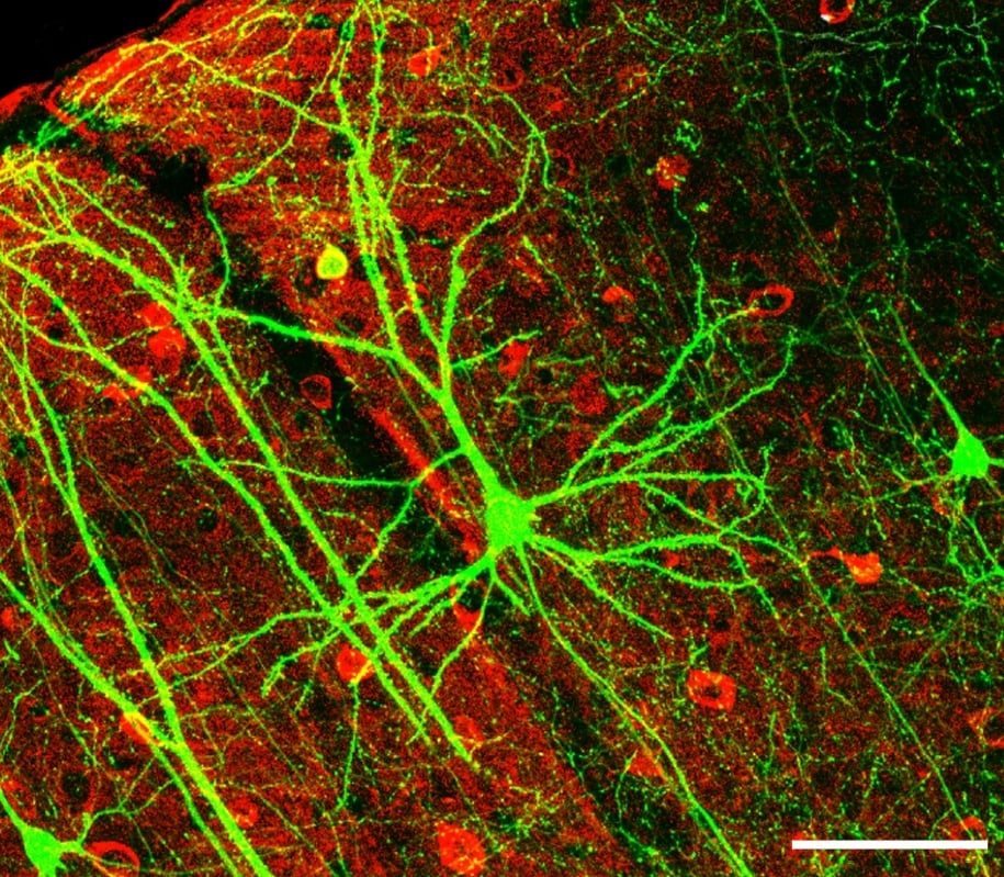
Why Hebbian Learning Matters in 2026
Hebbian learning matters because it is the answer to the question a wiring map cannot answer. A connectome gives you every path between neurons, but not how strong each path is. Plasticity is the process that sets those strengths, and Hebb's rule was the first serious guess at how. The complete connectome explainer makes the same point from the mapping side: wiring is necessary and not sufficient.
The rule is also being tested harder than ever. In March 2025, Antoine Madar and Mark Sheffield at the University of Chicago reported in Nature Neuroscience that the place cells of mice shift in ways that Hebbian spike-timing plasticity explained only in part. It covered the small, gradual shifts. A non-Hebbian rule called behavioral timescale synaptic plasticity (BTSP), which acts over seconds, covered the whole range. A 2026 ICML paper by Koplow, Poggio and Ziyin adds a warning from the AI side: weight decay alone can produce Hebbian-looking signatures, even with random updates. A signature that looks Hebbian does not prove a Hebbian mechanism.
The idea has also moved into agent design. HeLa-Mem, an April 2026 research paper, models the long-term memory of a language-model agent as a graph whose links strengthen through repeated co-activation. It reports gains on the LoCoMo benchmark with fewer context tokens. It is research, not a product, but it shows that "co-activation" is again a working term for people who build agent memory.
How Hebbian Learning Works
Hebb's actual words, from The Organization of Behavior (1949, p. 62), as reproduced on Wikipedia: "When an axon of cell A is near enough to excite a cell B and repeatedly or persistently takes part in firing it, some growth process or metabolic change takes place in one or both cells such that A's efficiency, as one of the cells firing B, is increased." The key phrase is takes part in firing it. That is causation and order, not only co-occurrence.
- A weak synapse exists. Cell A connects to cell B, but a single spike from A barely moves B.
- A fires just before B. A's spike arrives a few milliseconds before B fires, while other inputs are already pushing B toward its own spike.
- The NMDA receptor detects the coincidence. It opens only when glutamate from A arrives and B is depolarized, which lifts a magnesium block. Roger Nicoll's 2017 history of LTP in Neuron sets out this model: strong depolarization relieves the Mg2+ block of the NMDA channel, and calcium flows in. The receptor needs both cells at once, which makes it a coincidence detector.
- Repetition potentiates the synapse. Calcium enters, and the synapse strengthens. Bliss and Lømo showed this in 1973 in anaesthetized rabbits: repetitive trains of stimuli to the perforant path potentiated responses in the dentate area in 15 of 18 animals, for 30 minutes to 10 hours. That was long-term potentiation (LTP).
- Timing sets the sign. In 1997, Markram, Lübke, Frotscher and Sakmann reported in Science that the precise timing of an output spike relative to an input moved cortical synapses up or down. In 1998, Bi and Poo recorded pairs of cultured rat hippocampal neurons (Journal of Neuroscience). A postsynaptic spike within 20 ms after the input produced LTP. A spike within 20 ms before it produced long-term depression (LTD). Both needed NMDA receptors. This is spike-timing-dependent plasticity (STDP).
In a model neuron, the plain rule is one line, and its flaw fits in the next three:
Hebb's rule            Δw_ij = η · x_i · x_j
                       (η = learning rate, x_i and x_j = activity of the two cells)

Runaway feedback       strong w  →  more co-firing  →  larger Δw  →  stronger w  →  ...
                       with positive activity, nothing in the rule makes w smaller

Oja's fix (1982)       Δw = η · y · (x − y · w)      the extra term keeps |w| bounded
For positive activity, the plain rule only adds. Wikipedia's summary notes that with a dominant signal the weights grow or shrink exponentially. Erkki Oja's 1982 rule adds normalization, and a single neuron trained with it converges to the first principal component of its input. The brain has its own brakes: LTD, and the Bi and Poo finding that LTP occurred only at synapses that started relatively weak.
Hebbian Learning vs STDP vs Backpropagation
Hebbian learning is local: each synapse sees only the two cells it joins. Backpropagation is global: every weight is adjusted by an error signal computed at the output and sent back through the whole network. That difference is why AI moved on. The perceptron already used an error-corrected update in 1957, the Widrow-Hoff rule followed at Stanford a few years later, and backpropagation, popularized in 1986 by Rumelhart, Hinton and Williams in Nature, trained the hidden layers of the multi-layer networks behind deep learning.
| Question | Hebbian rule (1949) | STDP (1998) | Backpropagation (1986) |
|---|---|---|---|
| What changes a weight | Two connected cells active together | The order of two spikes, within about 20 ms | The gradient of an error at the output |
| Information used | Local: the two cells only | Local: the two cells plus spike timing | Global: the whole network and a target |
| Needs a right answer | No | No | Yes, a label or a loss |
| Can weaken a link | Only if activity can be negative | Yes, reversed order gives LTD | Yes, in either direction |
| Main failure | Runaway growth without normalization | Explains small shifts, not every change in vivo | Not known to be how a brain learns |
| Where it lives now | Associative memory, Hopfield networks | Spiking neural network models | Every large language model |
Hebb's rule did not disappear from AI. The Hopfield network (1982), part of the work behind the 2024 Nobel Prize in Physics for John Hopfield and Geoffrey Hinton, stores patterns with a Hebbian outer-product rule. The Nobel committee's popular explainer still calls Hebb's hypothesis one of the basic rules for updating artificial networks. Its capacity is small: about 0.138 patterns per neuron for the classical network, according to the Hopfield network entry. Error-driven training won the scale race because it learns what you asked for, not only what happened together.
Beyond Hebb: Three-Factor Rules and BTSP
Plain Hebbian learning has two factors: the activity of the sending cell and the activity of the receiving cell. That leaves a gap. Behavior unfolds over seconds, and a spike-timing window closes after about 20 ms, so a two-factor rule cannot connect an action to an outcome that arrives later.
Two lines of work fill that gap:
- Three-factor rules. Wulfram Gerstner and colleagues reviewed the evidence in 2018. Co-activity only marks a synapse with an eligibility trace. The weight changes later if a third signal arrives, such as a neuromodulator that reports reward, punishment, surprise, or novelty. The authors call these rules neoHebbian.
- Behavioral timescale synaptic plasticity (BTSP). Bittner, Magee and colleagues reported in Science in 2017 that place fields in hippocampal area CA1 can form in a single trial. Inputs that arrived seconds before or after a burst of complex spiking were potentiated, even though they were neither causal nor close in time to the output. The authors describe this as notably different from Hebbian plasticity.
The labels are still argued over. Bittner's group called BTSP non-Hebbian because the input did not take part in firing the output, which is Hebb's own test. Others fold it into the three-factor family. Either way, the timeline below shows the field moving from "use strengthens a link" toward "use marks a link, and something else decides".
| Year | Finding | Who | What it added |
|---|---|---|---|
| 1949 | Hebb's postulate in The Organization of Behavior | Donald Hebb | A causal, use-based rule |
| 1973 | Long-term potentiation in the dentate area | Bliss and Lømo | Physical evidence for lasting change |
| 1982 | Normalized Hebbian rule | Erkki Oja | A stable rule that finds the first principal component |
| 1982 | Associative memory network | John Hopfield | Hebbian storage in an artificial network |
| 1997 | Spike order moves synapses up or down | Markram, Lübke, Frotscher, Sakmann | Timing matters |
| 1998 | A 20 ms window for LTP and LTD | Bi and Poo | The asymmetric STDP window |
| 2017 | Place fields formed in one trial over seconds | Bittner, Magee and colleagues | BTSP, a seconds-long rule |
| 2018 | Eligibility traces and a third factor | Gerstner and colleagues | The neoHebbian framing |
| 2025 | BTSP beats STDP on place-field shifts | Madar, Sheffield and colleagues | Model rules tested against mouse place-cell data |
Connection to Taskade
Taskade does not change weights, and no part of Taskade learns on its own. The useful idea from Hebb for a builder is structural: things that are used together belong together. In a Taskade workspace you make those links deliberately. You connect the projects that describe one job, and you give a Taskade AI Agent those projects, files, and links as its knowledge. The agent reads that material before it acts, and it keeps context across chats with persistent memory.
This is the loop that Workspace DNA describes: Memory, Intelligence, and Execution. Projects hold the facts. Agents and Taskade EVE, the agent inside Taskade Genesis, read those facts and decide. Automations across 100+ bidirectional integrations do the work and write results back into projects. The connectome view at /connect/dna draws this as a wiring map, with projects and shared context in the association ring. The neuroscience terms there are a metaphor. The workspace gets sharper the more you use it because it holds more content, not because anything rewires itself.
What You Would Build in Taskade
You already know which documents travel together. The pricing sheet always goes out with the contract template. The onboarding checklist always gets opened with the security policy. That knowledge lives in people's habits, and it leaves when they do.
In Taskade you would describe a co-citation board. Each time a support agent resolves a ticket, it records in a project row which knowledge documents it used. A scheduled automation asks a second agent once a week to read those rows, find the pairs of documents that keep appearing together, and propose a cross-link or a merge. A person approves each proposal before anything changes. The links that get used together get surfaced together, and every link is one you can open, read, and delete.
This is the three-factor idea in plain workflow terms. Co-use only marks a pair. The human approval is the third signal that decides whether the link is kept. You can wire the weekly step with Taskade automations and give the reviewing agent the knowledge project through agent knowledge.
Describe yours and build it free →
Related Concepts
- Connectome: the wiring map, which gives paths but not strengths
- Perceptron: the 1957 learning machine with an error-corrected update
- Neural Network: weighted connections, where "synaptic efficacy" became "weight"
- Deep Learning: the error-driven successor that scaled
- Hopfield Network: associative memory built on a Hebbian rule
- Memory Consolidation: how the brain turns a fresh trace into a lasting one
- Continual Learning: why models find it hard to learn after training ends
- Agent Memory: how AI agents keep context across sessions
Frequently Asked Questions About Hebbian Learning
What is Hebbian learning in simple terms?
Hebbian learning is the rule that a connection gets stronger when it is used. If neuron A repeatedly helps make neuron B fire, the synapse from A to B becomes more effective. Donald Hebb proposed it in 1949, and later experiments on long-term potentiation confirmed the core of it.
Did Donald Hebb say "neurons that fire together wire together"?
No. Hebb never wrote that line. Carla Shatz used "cells that fire together wire together" in a September 1992 Scientific American article, and Siegrid Löwel and Wolf Singer printed a similar phrase in Science in January 1992, as Language Log documents. Hebb wrote about one cell taking part in firing another, which implies order, not only simultaneity.
What is the difference between LTP and STDP?
Long-term potentiation (LTP) is a lasting increase in synaptic strength after strong or repeated activity, first shown by Bliss and Lømo in 1973. Spike-timing-dependent plasticity (STDP) is a timing rule for when LTP or its opposite, LTD, occurs. In Bi and Poo's 1998 study, input that arrived within about 20 ms before the output spike gave LTP, and input within about 20 ms after it gave LTD.
What is the formula for Hebbian learning?
The basic form is Δw = η · x_i · x_j. The weight change equals a learning rate times the activity of the two connected units. With positive activity it has no term that makes weights smaller, so the weights grow without bound. Variants such as Oja's rule (1982) add normalization to keep the weights stable.
What is behavioral timescale synaptic plasticity (BTSP)?
BTSP is a plasticity rule found in the hippocampus. Bittner and colleagues reported in 2017 that inputs arriving seconds before or after a burst of complex spiking were strengthened in a single trial, which is far outside the 20 ms STDP window. A 2025 Nature Neuroscience study by Madar and Sheffield found that BTSP explained the full range of place-field shifts in mice, while STDP explained only the small, gradual ones.
Is Hebbian learning the same as backpropagation?
No. Hebbian learning is local and needs no correct answer. Each connection updates from the two units it joins. Backpropagation is global and needs a target. It computes an error at the output and sends it back to adjust every weight. Modern language models are trained with backpropagation.
Why did AI stop using Hebbian learning?
Because it learns correlation, not a goal. A Hebbian network strengthens whatever happens together, whether or not that helps with a task, and the plain rule is unstable. Error-driven rules, from the perceptron to backpropagation, learn what you ask for, which is what made large trained networks possible.
Is Hebbian learning still used in AI?
Yes, in narrower places. Hopfield networks store patterns with a Hebbian rule, spiking neural network models use STDP, and 2026 research such as HeLa-Mem uses Hebbian co-activation to organize agent memory as a graph. The large models you use every day are trained with backpropagation.
Do Taskade AI agents rewire themselves like neurons?
No. Taskade agents do not change their own weights or learn on their own. They read the projects, files, and links you give them, and they keep context across chats with persistent memory. What improves over time is the content they read, which you can open, edit, and delete. See Taskade AI Agents.