




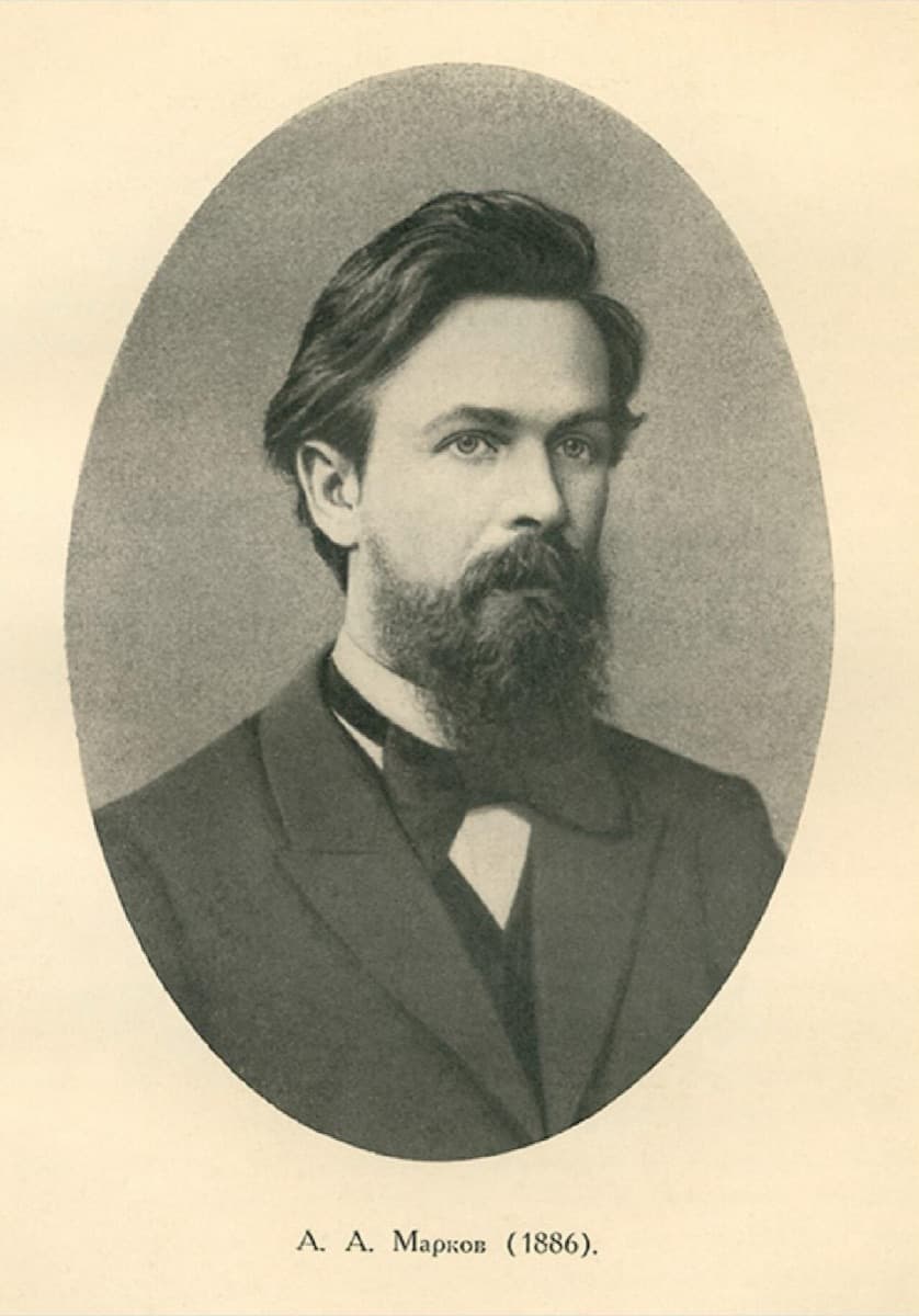
In 1905, Russia was in revolt, and its mathematicians took sides. On one side stood Pavel Nekrasov, a deeply religious professor sometimes called the Tsar of Probability, who had built a statistical argument that human free will was scientifically demonstrable. On the other stood Andrey Markov, an atheist so combative that colleagues called him Andrey the Furious, who filed Nekrasov's work under a category he named in print: the abuses of mathematics.
To demolish the argument, Markov needed to invent something. He sat down with the first 20,000 letters of Pushkin's Eugene Onegin and counted them by hand.
What came out of that counting is now the mathematics behind Google's original ranking algorithm, the simulation method that reshaped nuclear weapons design after the war, the models that predict customer churn, and a live 2026 argument about whether ChatGPT is anything more than a very expensive version of the same idea.
TL;DR: A Markov chain predicts the next state using only the current state, throwing away all earlier history. That single simplification makes impossible systems tractable, which is why it powers PageRank, Monte Carlo simulation, and the probability layer inside every language model. A 2024 proof showed that an autoregressive model with a 128,000 token window is formally a Markov chain, with a state space of more than 10^678,000. Build a live state tracker in Taskade.
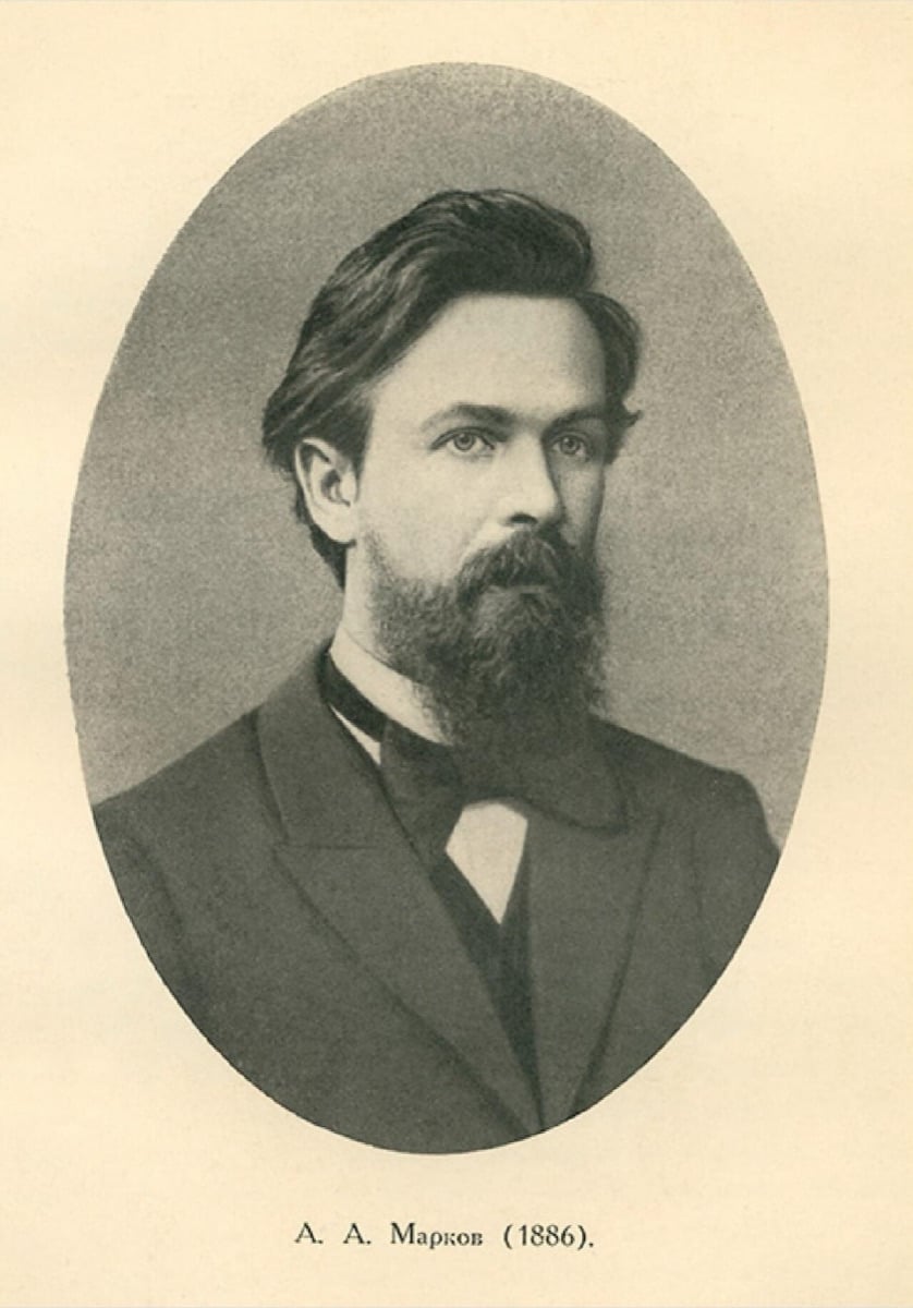
Andrey Andreyevich Markov, photographed in 1886. He described his own interest in applications with complete indifference, then produced the tool half the internet runs on. Image: Wikimedia Commons, public domain.
What Is a Markov Chain?
A Markov chain is a system that moves between a fixed set of states, where the probability of each next move depends only on the current state and not on the path taken to reach it. It has exactly three ingredients: states, transitions, and probabilities. Nothing else. The probabilities leaving any single state must sum to 1, because the system has to be somewhere next.
Here is a complete Markov chain. A coffee shop serves exactly one special per day, and tomorrow's special depends on today's.
That diagram is the entire object. Every arrow carries a probability, every state's outgoing arrows add to 1.00, and the arrows that loop back to the same state are just as real as the ones that leave.
| Ingredient | What it is | In the coffee shop | The rule you cannot break |
|---|---|---|---|
| States | The possible configurations | Espresso, Latte, Cold Brew | The system is in exactly one at a time |
| Transitions | Directed arrows, including self-loops | Espresso to Latte, Latte to Latte | Missing arrow means probability zero |
| Probabilities | A weight on each arrow | 0.60 for Espresso to Latte | Every state's outgoing weights sum to 1 |
The sum-to-one rule is the first thing to check when a hand-built chain misbehaves. A row that adds to 0.97 is not a rounding annoyance. It is a leak, and it quietly drains probability out of your model over enough steps.
The question a Markov chain answers
Given where the system is now, what is it likely to be doing in one step, in ten steps, and in the long run forever? Those three questions have three different answers, and the rest of this article is how to get each one.
The Markov Property: What "Memoryless" Actually Means
The Markov property says the conditional distribution of the next state, given the entire history, equals the conditional distribution given only the most recent state. In notation:
P(X(n+1) = j | X(n), X(n-1), ..., X(1), X(0)) = P(X(n+1) = j | X(n))
Suppose the coffee shop served Latte, then Espresso, then Latte. What is the chance of Cold Brew tomorrow? Read the Latte row, take 0.60, and stop. Days one and two are not discounted or down-weighted. They are discarded.
Two clarifications, because both get muddled constantly.
Memorylessness is not amnesia. It does not claim the past had no effect. It claims the past's entire effect is already carried inside the present state. If something in the history matters and the state does not capture it, your state definition is wrong, not the mathematics.
"Memoryless" is an overloaded word. The memoryless property of the exponential and geometric distributions (a lightbulb that has burned for 500 hours is no more likely to fail in the next hour than a new one) is a related but separate idea about waiting times. The Markov property is about state sequences. They share a word and get conflated in search results constantly.
What a non-Markov process looks like
The cleanest counterexample is counting cards in blackjack. The chance the next card is an ace depends on every card already dealt, not just the card face-up on the table. Drawing without replacement is inherently non-Markov with respect to the visible card.
| Process | Markov with respect to the obvious state? | Why |
|---|---|---|
| Dice rolls | Yes, trivially | The next roll ignores everything, including the current state |
| Weather (sunny, rainy) | Approximately | Yesterday adds a little signal, but not much |
| Blackjack, visible card | No | Depends on the whole discard pile |
| A runner's next mile | No | Accumulated fatigue is not in "current pace" |
| Stock price level | Roughly, by design | The efficient-market claim is literally a Markov claim |
| A support ticket's status | Usually yes | Status genuinely summarizes what happens next |
The escape hatch that makes the property nearly universal
Enlarge the state until it holds everything that matters. Blackjack becomes Markov the moment the state is the full count of remaining cards instead of the face-up card. Weather becomes more Markov when the state is a pair of consecutive days rather than one day. A runner becomes Markov when the state includes distance covered.
This move is the single most important practical technique in the whole subject, and it recurs in every section below. When the Manhattan Project modeled neutrons, they put position, velocity, and energy into the state. When Claude Shannon modeled English, he moved from one previous letter to two, and then to whole words. When a modern language model takes a context window of 128,000 tokens, that window is the enlarged state.
The cost is always the same: the state space explodes. Section 11 shows exactly how far that explosion goes.
How to Read a Transition Matrix
A transition matrix is the chain written as a grid, where the entry in row i and column j is the probability of moving from state i to state j in one step. Rows are "from," columns are "to," and every row sums to 1.
For the rest of this article we will use a smaller example so every number stays checkable by hand. Two states, sunny and rainy.
              TO
           Sunny   Rainy      row sum
      +-------------------+
F  S  |   0.80    0.20    |    1.00
R  u  |                   |
O  n  |                   |
M  y  |                   |
      |                   |
   R  |   0.40    0.60    |    1.00
   a  |                   |
   i  |                   |
   n  |                   |
   y  +-------------------+
Why matrix multiplication is secretly path-counting
Start on a sunny day. What is the weather two days from now? Do it the long way, by listing every path:
| Path | Probability | Ends |
|---|---|---|
| Sunny to Sunny to Sunny | 0.8 x 0.8 = 0.64 | Sunny |
| Sunny to Rainy to Sunny | 0.2 x 0.4 = 0.08 | Sunny |
| Sunny to Sunny to Rainy | 0.8 x 0.2 = 0.16 | Rainy |
| Sunny to Rainy to Rainy | 0.2 x 0.6 = 0.12 | Rainy |
Add the paths that end sunny: 0.64 + 0.08 = 0.72. Add the paths that end rainy: 0.16 + 0.12 = 0.28.
That hand calculation is exactly the first row of the matrix squared. Matrix multiplication sums over every intermediate state, weighted by probability, automatically. To find the distribution after n steps, raise the matrix to the power n, and you never enumerate a path again.
For a 2-state chain this is a party trick. For a chain with billions of states, which is what Google built, it is the difference between a computation and an impossibility.
The row vector convention
Track the current distribution as a row vector. If today is definitely sunny, that vector is [1, 0]. Multiply it by the matrix and you get tomorrow's distribution. Feed the answer back in and you get the day after.
[1, 0]  x  A  =  [0.80, 0.20]         after 1 day
[0.80, 0.20] x A  =  [0.72, 0.28]     after 2 days
[0.72, 0.28] x A  =  [0.688, 0.312]   after 3 days
Watch the second column. It is drifting toward something.
The Stationary Distribution: Where Every Chain Ends Up
The stationary distribution is the one probability distribution that stops changing when you apply another step of the chain. Written as an equation, if the distribution is the row vector pi, then pi times A equals pi. For our weather chain, that distribution is 2/3 sunny and 1/3 rainy, and the chain converges to it from any starting point.
There are two ways to find it, and you should know both because they answer different questions.
Method 1: simulate and count
Walk the chain for a very long time and tally the fraction of steps spent in each state. This is legitimate, it is the oldest method, and it is what Monte Carlo turns into a discipline. It has two weaknesses worth knowing: its error shrinks only as the square root of the sample count, so ten times the work buys about three times the precision, and it can never tell you whether the answer is unique.
Method 2: solve the eigenvector equation
pi A = pi is the eigenvector equation Av = λv with λ set to 1 and the multiplication order reversed. In words: the stationary distribution is a left eigenvector of the transition matrix with eigenvalue 1. Add the constraint that the entries sum to 1, solve the small linear system, and you are done exactly, in closed form, with no simulation.
For the weather chain, solving gives pi = [2/3, 1/3] = [0.6667, 0.3333]. Check it:
0.6667 x 0.8  +  0.3333 x 0.4  =  0.5333 + 0.1333  =  0.6667   (sunny)
0.6667 x 0.2  +  0.3333 x 0.6  =  0.1333 + 0.2000  =  0.3333   (rainy)
And here is what the algebra gives you that simulation cannot: count the eigenvectors with eigenvalue 1. Exactly one means a unique long-run answer. More than one means the chain has genuinely separate regimes and where you start decides your fate permanently. No amount of walking reveals that.
Watching the matrix forget
Raise the matrix to higher powers and something specific happens to the rows.
| Power | Row "from Sunny" | Row "from Rainy" | Rows differ by |
|---|---|---|---|
| A^1 | 0.8000, 0.2000 | 0.4000, 0.6000 | 0.4000 |
| A^2 | 0.7200, 0.2800 | 0.5600, 0.4400 | 0.1600 |
| A^3 | 0.6880, 0.3120 | 0.6240, 0.3760 | 0.0640 |
| A^5 | 0.6701, 0.3299 | 0.6598, 0.3402 | 0.0102 |
| A^10 | 0.6667, 0.3333 | 0.6666, 0.3334 | 0.0001 |
The two rows start clearly different, because starting sunny genuinely is different from starting rainy. Then they converge until they are identical to four decimal places.
When every row of A^n is the same, the chain has forgotten where it started. That limiting row is the stationary distribution. Hold onto this idea, because in the section on mixing time we will look at a case where forgetting the starting point is the bug, not the theorem.
Here is the same convergence from both starting states:
One line starts at certainty and one starts at zero. Within eight steps they are indistinguishable at 66.7 percent. The gap between them shrinks by a constant factor of 0.4 every single step, and that number turns out to be the second eigenvalue of the matrix. That is the whole theory of convergence speed in one observation.
Limiting distribution vs stationary distribution
These two get used interchangeably and they are not the same thing. This is one of the most-viewed unanswered questions in the entire topic, so here is the clean version.
| Stationary distribution | Limiting distribution | |
|---|---|---|
| Definition | A distribution unchanged by one step: pi A = pi | What the distribution converges to as steps go to infinity |
| Always exists? | Yes for any finite chain | No |
| Unique? | Not necessarily | Yes if the chain is irreducible. A reducible one can have a different limit for each starting state |
| Depends on start? | No | No for an irreducible chain. A reducible one can settle in different places depending on where it began |
| Relationship | Every limiting distribution is stationary | Not every stationary distribution is a limit |
The counterexample that makes it click: a chain that flips A to B to A to B with probability 1. Its stationary distribution is 50-50, and you can verify that algebraically. But it never converges to 50-50, because at every individual step the system sits entirely in one state. Start at A and you are at A on every even step, full stop. The stationary distribution is real and the limit does not exist.
That gap is exactly the aperiodicity condition, which is next.
When Does a Chain Settle? Irreducible and Aperiodic, Diagnosed
A finite Markov chain has a unique stationary distribution that it converges to from any starting point when it is both irreducible and aperiodic. Most textbooks define these two words and move on. What people actually need is how to diagnose them in a chain they built themselves, so here are both tests.
Irreducible: can everything reach everything?
Irreducible means every state can eventually reach every other state, in any number of steps, following arrows with non-zero probability.
The test is a reachability search. Pick any state, follow every outgoing arrow repeatedly, collect everything reachable. If that set is not all states, the chain is reducible. Then start from something you reached and check you can get back.
Both of those are reducible, for different reasons, and the difference matters. Two disconnected components means two separate long-run answers and your starting state is destiny. A one-way trap is an absorbing state, which is not a modelling error at all. It is often the entire point, and section 12 is built on it.
Why you should care in product terms: an absorbing state you did not intend is one of the highest-severity bugs a system can have. It is a state a user can enter and never escape. Running this test on your own state machine finds them systematically instead of by customer complaint.
Aperiodic: does the chain cycle on a fixed rhythm?
A state has period k if every possible return to it happens on a multiple of k steps. Period 1 means aperiodic.
The shortcut that covers almost every real case: one self-loop is enough. If any state has a non-zero chance of staying put for a single step, that state has period 1, and in an irreducible chain the whole chain inherits it. This is why that little arrow curling back on itself in a diagram matters far more than it looks.
Left chain: start at Billed and you are at Billed on every even step and Reconciled on every odd step, forever. Right chain: add a single 10 percent chance of staying, and the rhythm breaks immediately and it converges.
A chain that is both irreducible and aperiodic is called ergodic, which answers another commonly asked question. Ergodic requires both conditions, not just irreducibility.
| Diagnosis | Test | If it fails |
|---|---|---|
| Rows sum to 1 | Add each row | You have a probability leak |
| Irreducible | Reachability search from any state | Multiple long-run answers, or an absorbing trap |
| Aperiodic | Look for any self-loop | Probabilities cycle instead of settling |
| Ergodic | Both of the above | The limit may not exist |
How to Build a Transition Matrix From Your Own Data
Every tutorial hands you a transition matrix. Almost none shows how to make one, and that single missing step is what separates a reader who understood the article from one who can use it. The method is counting and dividing. Count observed transitions, then divide each count by its row total.
Take a subscription business. Define three states: Trial, Paid, Churned. Pull the event log, sort by customer and month, and turn each customer's history into a sequence like Trial, Trial, Paid, Paid, Paid, Churned. Then count every consecutive pair.
Step 1: the raw counts.
| From \ To | Trial | Paid | Churned | Row total |
|---|---|---|---|---|
| Trial | 400 | 350 | 250 | 1,000 |
| Paid | 0 | 3,290 | 210 | 3,500 |
| Churned | 0 | 0 | 500 | 500 |
Step 2: divide each row by its total.
| From \ To | Trial | Paid | Churned |
|---|---|---|---|
| Trial | 0.40 | 0.35 | 0.25 |
| Paid | 0.00 | 0.94 | 0.06 |
| Churned | 0.00 | 0.00 | 1.00 |
Every row sums to 1 automatically, because you divided by the row total. That is the whole procedure, and it is exactly what Markov did by hand in 1913.
Four things to get right
- Pick a fixed time step and stick to it. Monthly transitions and weekly transitions produce different matrices for the same business. The matrix is only meaningful alongside its step size.
- Include self-transitions. "Stayed in Trial" is a real observation and dropping it inflates every other probability in the row.
- Watch thin rows. A row built from 12 observations produces probabilities you should not trust. A row built from 3,500 is solid. This is ordinary sample-size discipline and it is where most homemade models go wrong.
- Check the Markov property before you trust the answer. Split the data by history. If customers who reached Paid from a long trial churn at a visibly different rate than those who converted immediately, then the state "Paid" is not summarizing what matters, and you need to split it, for example into "Paid, converted fast" and "Paid, converted slow." That is the enlarge-the-state move again.
That fourth check is the one people skip, and it is the difference between a model and a decoration. It is the same discipline that goes into good predictive analytics generally.
The Feud That Invented the Markov Chain
Markov chains exist because of a fight about free will. In 1913, Andrey Markov published an analysis of 20,000 letters from Eugene Onegin specifically to destroy an argument by Pavel Nekrasov, and the tool he built for the demolition outlived the argument by a century.
The 200-year-old assumption
Jacob Bernoulli proved the law of large numbers in 1713: run enough independent trials and the average outcome approaches the expected value. Flip a fair coin ten times and you might see six heads. Flip it a hundred times and you land near 51-49. The ratio thrashes early and settles late.
Bernoulli proved it for independent events. Ask a room to privately estimate an item's value and average the guesses, and you converge near the truth. Ask them to shout the answers out loud in turn, and the first speaker's number anchors everyone after. The guesses are now dependent, and the average converges to something, just not to the truth.
Nekrasov's mistake
Nekrasov's argument ran like this:
- Independence gives you the law of large numbers.
- Belgian marriage counts from 1841 to 1845 hovered near 29,000 a year. Crime rates and birth rates behaved similarly.
- So those statistics obey the law of large numbers.
- So the underlying events must be independent.
- Those events are human decisions, to marry, to commit a crime, to have a child.
- Therefore free will is a measured scientific fact.
Step 4 is where it dies. Independence being sufficient for convergence does not make it necessary. To close that gap Nekrasov needed to prove no dependent process could converge. He never did, because it is false.
Eugene Onegin, counted by hand
Markov needed a system where dependence was undeniable, so he chose text. Whether the next letter is a vowel or a consonant obviously depends on the current one. He stripped punctuation and spaces from the first 20,000 letters of Pushkin's novel in verse and counted: 43 percent vowels, 57 percent consonants. Then he counted overlapping pairs.
| Pair | If letters were independent | What Markov actually counted | Verdict |
|---|---|---|---|
| Vowel then vowel | 18.5% | 6% | Three times too rare |
| Vowel then consonant | 24.5% | 37% | Far too common |
| Consonant then vowel | 24.5% | 37% | Far too common |
| Consonant then consonant | 32.5% | 20% | Far too rare |
Dependence, established empirically, by hand, on paper. Then he built the machine by dividing joint counts by marginals, exactly the procedure in the previous section: the vowel-to-vowel probability is the vowel-vowel pair frequency divided by the vowel frequency, which comes out near 0.13. (The percentages in the table are rounded to whole numbers, so dividing them directly gives 0.14. Markov worked from the raw counts.)
Then he ran it. Start at a vowel, draw a random number, follow the arrow, repeat, and track the running ratio. It thrashed, then converged to 43 percent vowels and 57 percent consonants, the exact split he had counted by hand.
A demonstrably dependent system obeying the law of large numbers. Nekrasov's step 4 was dead. Markov closed the paper with a line that reads like a door slamming:
"Thus, independence of quantities does not constitute a necessary condition for the existence of the law of large numbers."
The lesson that outlived the fight
Convergence is not evidence of independence. A metric that has settled into a stable average tells you nothing about whether the underlying units act independently. Stable conversion rate, stable churn, stable latency, stable pass rate: every one is equally consistent with a strongly coupled system. Any argument shaped like "the number is steady, so the parts must be behaving independently" is Nekrasov's argument, and it is still being made in dashboards today.
Markov himself did not care what any of it was for. He wrote: "I am concerned only with questions of pure analysis. I refer to the question of the applicability with indifference." The result was largely ignored at the time.
Monte Carlo: How a Card Game Helped Build the Bomb
Monte Carlo simulation is what you do when a system has too many possible outcomes to enumerate: instead of computing the answer, you sample random outcomes and count. It was invented in 1946 by Stanislaw Ulam while he was recovering from encephalitis and playing solitaire, and it became the method that carried postwar weapons design. Wartime critical mass had already been settled by deterministic diffusion theory; the first Monte Carlo runs on ENIAC did not happen until April 1948.
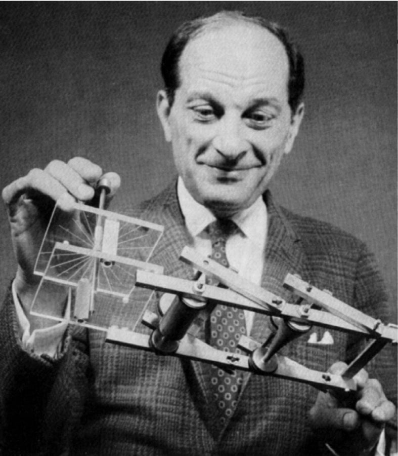
Stanislaw Ulam holding the FERMIAC, a mechanical device built to trace neutron histories through a reactor by hand. Image: Los Alamos National Laboratory via Wikimedia Commons, public domain.
The solitaire insight
Ulam wondered what fraction of randomly dealt solitaire games are winnable. A 52 card deck has 52 factorial arrangements, roughly 8 x 10^67, so an exact analysis is hopeless. Then the flash: do not solve it, sample it. Play a few hundred games, count the wins, and you have a statistical approximation of an analytically impossible number.
Von Neumann's correction, which is the actual method
Ulam brought the idea back to Los Alamos. John von Neumann saw immediately that it worked and that it did not transfer directly. Solitaire deals are independent: one game tells you nothing about the next. Neutrons are not. A neutron's behavior depends on where it is, how fast it is moving, and what it has already done.
You cannot draw independent samples from a dependent process. What you need is a Markov chain.
With one important wrinkle: the transition probabilities are not constant. They depend on the neutron's position, velocity, and energy, and on the geometry and mass of the assembly. A fast neutron might be 30 percent scatter, 50 percent absorbed or escaped, 20 percent fission. A slower one has different numbers. This is a Markov chain over a rich state, which is the enlarge-the-state move from section 2 applied under wartime pressure.
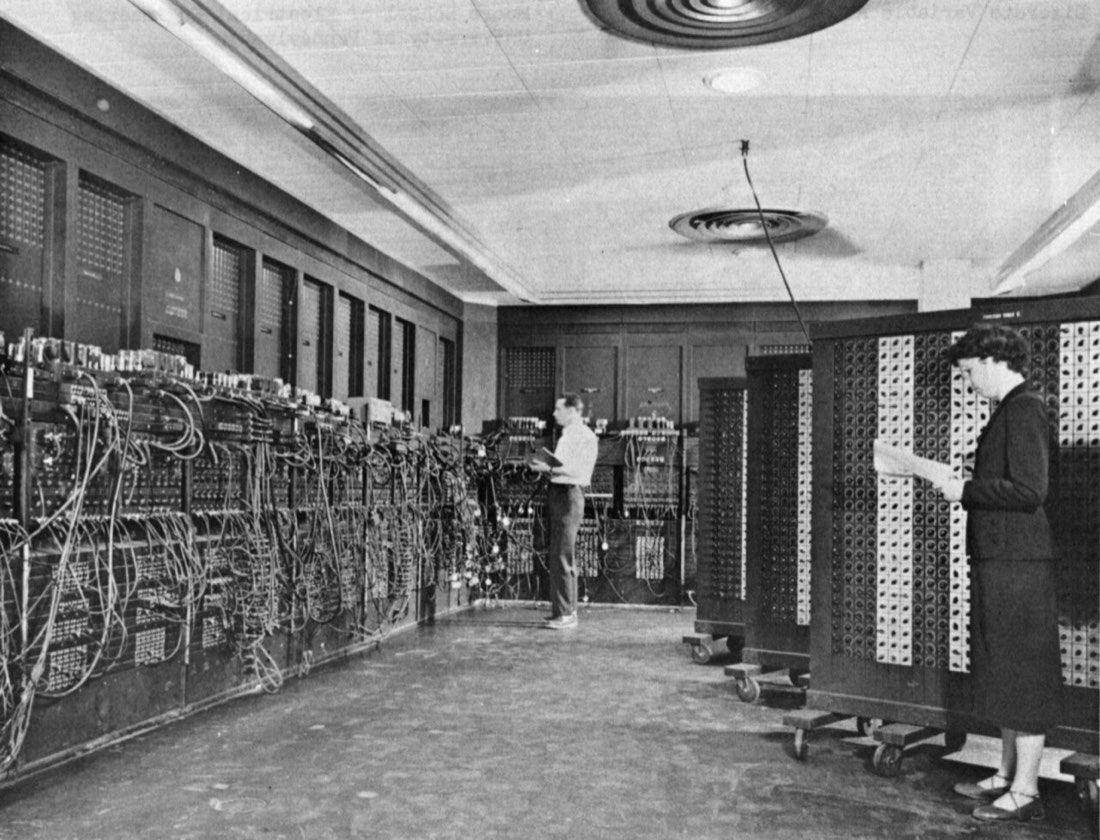
The ENIAC at the Ballistic Research Laboratory. The first Monte Carlo neutron runs were executed here. Image: US Army via Wikimedia Commons, public domain.
Reading the answer off a histogram
They ran the chain on ENIAC across seven problems, each carrying a population of about a hundred neutrons through successive censuses and recording alpha, the neutron growth rate.
| Value of k | What it means physically | What you have built |
|---|---|---|
| k < 1 | Each generation is smaller than the last | The reaction dies out |
| k = 1 | Each generation replaces itself exactly | A self-sustaining reactor |
| k > 1 | Each generation is larger | Exponential growth, a bomb |
The whole method is: approximate answers to equations too hard to solve directly, by walking a chain and tallying. Ulam's uncle gambled at the Monte Carlo Casino in Monaco, the random sampling and the stakes rhymed, and the name stuck. By late 1948 Argonne was using it for reactor design.
Markov chain Monte Carlo, explained without Bayes' theorem
MCMC is the most searched and worst explained topic in this subject, so here it is in plain terms.
Some questions have too many possible answers to check one by one, and the answers are not equally likely. MCMC builds a random walk whose rules make it spend more time in likely regions and less in unlikely ones. Let it wander long enough, and the fraction of time spent in each region approximates that region's true probability. You never enumerate anything. You just walk and count.
The trick that makes it work is the one from section 4 read backwards. Normally you have a chain and you want its stationary distribution. In MCMC you want a particular distribution, so you design a chain whose stationary distribution is the one you want, then run it. The Metropolis algorithm, published in 1953 by the same Los Alamos circle, is the recipe for designing that chain. Every modern Bayesian statistics tool is built on this idea, and "how long do I have to run it" is a mixing-time question, which is section 13.
PageRank: Google Turned the Web Into a Markov Chain
PageRank scores a web page by the fraction of time a random surfer clicking links at random would spend on it, which is precisely the stationary distribution of a Markov chain over the web graph. It was the single technical idea that let Google beat Yahoo, and it is a direct application of everything above.
The problem in 1998
The search engines of the era, Excite and Lycos among them, ranked by term frequency: how often your query words appear on the page. That had an obvious exploit, and it was exploited immediately, by repeating keywords hundreds of times in white text on a white background. The engines had a notion of relevance but no notion of quality.
Sergey Brin and Larry Page borrowed the intuition from library cards: a book stamped with many due dates is probably a good book. A link is an endorsement. And crucially, the more links a page hands out, the less each of its endorsements is worth.
A four-page web, worked all the way through
Pages are states, links are transitions, and a page with n outgoing links sends the surfer down each with probability 1/n.
Amy links only to Ben, so that arrow carries probability 1. Ben links to three pages, so each gets 1/3. Chris links to two, so each gets 1/2. Dan links to two, same. Solve pi A = pi and you get the exact answer:
| Rank | Page | Share of the surfer's time | Inbound links | Why |
|---|---|---|---|---|
| 1 | Ben | 41.4% (12/29) | 3 | Everyone links to Ben |
| 2 | Amy | 24.1% (7/29) | 2 | Fewer links, but one is from Ben |
| 3 | Dan | 20.7% (6/29) | 2 | Two links, both diluted |
| 4 | Chris | 13.8% (4/29) | 1 | Only Ben points here, and Ben splits three ways |
Notice that Amy and Dan both have two inbound links and do not tie. The vote is weighted by the voter's own score, recursively. That is the entire anti-spam property, and it falls out of the math rather than being bolted on.
Why a hundred fake pages pointing at you does very little
Spin up 100 pages that all link to your site. For the first few steps of the walk they inflate your number. But nothing links to them, so the random surfer almost never arrives there in the first place, and over many steps their contribution shrinks to the teleport mass every page receives. It does not fall to zero, which is why link farms were worth building at all and why Google spent years fighting them. What changes is the economics: you need enormously more fake pages to move the number, and the stationary distribution can tell many links from quality links.
Damping: a theorem that became a product decision
The real web is not irreducible. It has dead ends and traps, so the conditions in section 6 fail and there is no unique answer to converge to. The fix: 85 percent of the time follow a link, 15 percent of the time teleport to a random page.
Any damping factor below 1 forces irreducibility and aperiodicity, which is what guarantees a unique stationary distribution reachable from any start. The specific value is tuning: Brin and Page simply wrote that they "usually set d to 0.85" and gave no derivation. A theorem about existence dictated the shape of the parameter, and a judgement call fixed its value.
What this still means if you run a website
Four practical consequences, all direct from the math:
- Outbound links divide your vote. A hub page linking to 40 things passes about 1/40 of its own score to each. The 41st link dilutes the other 40.
- Pages that link nowhere are sinks. They absorb score and pass none back. They are literally the dead ends damping was invented to paper over.
- A link's value is the linker's own score. Getting linked from a page nothing links to is worth close to nothing.
- Your own internal link structure is a Markov chain you control, and you can compute its stationary distribution yourself to see whether your score concentrates where you want it. Most sites have never checked.
The history is in 50 years of computing primitives and the full computing timeline. The graph thinking behind it lives on in knowledge graphs and how AI agents use them.
Are Large Language Models Just Markov Chains?
Formally yes, and practically no, and the gap between those two answers is the most interesting thing in this article. In 2024, researchers Zekri, Odonnat, Benechehab, Bleistein, Boullé and Redko published Large Language Models as Markov Chains, proving the equivalence precisely. The proof is real. The conclusion people draw from it is usually wrong.
The formal claim, stated exactly
An autoregressive model reads a context window and emits a probability distribution over the next token. Nothing outside that window influences the output. So define the state as the entire context window, and the process is Markov by construction: the next state depends only on the current one.
The paper gives the size of that state space for a vocabulary of T tokens and a window of K: the number of sequences of length at most K, which is T(T^K - 1)/(T - 1), on the order of T^K. It also proves the resulting chain is ergodic and admits a unique stationary distribution.
Now put real numbers in. A vocabulary of about 200,000 tokens and a context window of 128,000 tokens:
        States in the LLM chain:   ~10^678,000
                                   (a 1 followed by 678,000 zeros)  Atoms in the observable universe:  ~10^80
Seconds since the Big Bang:  ~10^17
States in our weather chain:  2
The equivalence is a statement about structure, not a usable description. Calling a language model a Markov chain is true in the same way that calling a novel "a sequence of characters" is true.
Four reasons the label is not the insight
| The claim | Why it is technically right | Why it does not explain anything |
|---|---|---|
| "It only looks at the current state" | The context window is the state | The state is 128,000 tokens of arbitrary history |
| "It has a transition matrix" | Formally yes | It has more entries than the universe has atoms, and it is never materialized |
| "It has a stationary distribution" | Proved, and it is unique | Reaching it means generating until the output degenerates, which is a failure mode, not a use case |
| "So it is just statistics" | All prediction is statistics | The content is in how the probabilities are computed |
Attention is the part that is not Markov-shaped
A classical Markov chain of order n stores one independent probability row for every possible window. It is maximally expressive over that window and hopelessly data-hungry, because nothing it learns about one context transfers to another. The attention mechanism inside a transformer computes the same conditional distribution as a learned function of the window, deciding per token and based on content which parts of the history to weigh heavily.
In the phrase "the structure of the cell," earlier context like mitochondria or prison determines which meaning of cell the model uses. A tabular order-n chain could represent that too, if both words fell inside the window and you had seen every window often enough to estimate it. The difference is not what can be represented. It is what can be learned from finite data.
Both diagrams describe processes that are technically Markov over their windows. Only one of them learned which parts of the past deserve attention. That difference is the entire architecture, and it is covered properly in how large language models work.
Claude Shannon already ran this experiment
In the 1940s, Shannon picked up Markov's text idea and asked what happens if the state is bigger than one letter.
| State | Sample output | What it shows |
|---|---|---|
| One letter | Statistically correct nonsense | Right frequencies, no words |
| Two letters | Fragments like "whey", "of", "the" | Real words start appearing |
| Whole words | "attack on an English writer that the character of this point is therefore another method" | Runs of about four words make sense |
Shannon's observation is the scaling law in embryo: grow the state, grow the horizon of sense. A 128,000 token window is that same escalation carried to its limit. The information-theoretic half of this story, including why training loss is measured in bits, is in what cross-entropy really measures.
The temperature result nobody quotes
Read this one with its scope in view. The figures below come from the paper's toy model: a two-symbol vocabulary, a three-token window, and a 14 by 14 transition matrix trained on 37 examples. The plotted quantity is the smallest entry of that matrix raised to the window length, which is what drives their convergence bound. It is an illustration of the mechanism, not a measurement of a production language model.
The same 2024 paper measured how fast the chain converges, and found the temperature setting controls it directly:
| Temperature | Steps to reach the stationary distribution | What you see |
|---|---|---|
| 2.0 | About 30 | Converges fast into high-entropy noise |
| 1.0 | About 300 | Normal generation |
| 0.2 | Still not converged after 10^6 steps | Gets stuck, repeats itself |
This is a mathematically precise account of a thing every user has observed. Low temperature produces repetition loops, high temperature produces incoherence. Both are statements about the mixing behavior of a chain. If you have ever wondered why the same prompt gives different answers, the mechanics are in non-determinism in AI.
The 2026 twist: the frontier is getting more Markovian, not less
Here is the part that inverts the usual story. Diffusion language models, one of the most active research directions of 2026, generate text by starting from a fully masked sequence and unmasking it over a series of denoising steps. That corruption process is explicitly defined as a forward Markov process over discrete states, whose end point is an absorbing mask state, and generation learns the reverse dynamics.
So the standard narrative, that transformers broke the Markov assumption and we moved on, is not what actually happened. Attention broke the fixed-weight window. The frontier then went and built a new generation of models whose entire sampling procedure is an explicitly declared Markov process. The idea keeps coming back because it is the right abstraction for "a system that evolves one step at a time."
For the record, the first text generators to go viral on the public internet were literal Markov chains. Reddit's SubredditSimulator, which appears in the history of Moltbook and OpenClaw, was bots generating posts with Markov chains years before anyone had heard of a transformer.
Absorbing Chains: Churn, Retries, and Model Collapse
An absorbing state is one you can enter but never leave, and a chain with at least one is called an absorbing chain. This variant answers different questions from the ones above: not "where does the system settle" but "how long until it stops, and where does it stop?" Three important things share this exact shape.
Application 1: customer lifetime value
Take the subscription matrix built back in section 7. Churned is absorbing. The two questions worth money are how long a customer lasts and what fraction of trials ever convert.
Expected months as a paying customer, once someone converts, is 1 divided by the monthly churn probability: 1 / 0.06 = 16.7 months. At $10 a month that is about $167 of expected revenue per conversion.
Expected value of a new trial takes one more step. Collect the transient states into a matrix Q, then compute the fundamental matrix N = (I - Q)^-1, whose entries give the expected number of visits to each state. For this chain it works out to 1.67 expected months in Trial and 9.72 expected months in Paid, so a new trial signup is worth about $97 before you know anything else about them.
Probability a trial ever converts is 0.35 / (0.35 + 0.25) = 58.3 percent, because from Trial you either stay, convert, or churn, and staying just repeats the same gamble.
Three numbers a business would pay for, from counting transitions and inverting a 2x2 matrix. This is the part of the subject that most articles skip entirely, and it is arguably the most useful.
Application 2: retries, and why "mostly working" is a trap
Any process that retries on failure is an absorbing chain where success and permanent failure are the absorbing states. With per-attempt failure probability p, the expected number of attempts is 1 / (1 - p), and that number explodes.
| Per-attempt failure rate | Expected attempts | Practical reading |
|---|---|---|
| 10% | 1.11 | Barely noticeable |
| 25% | 1.33 | Fine |
| 50% | 2.00 | Double the load |
| 75% | 4.00 | Now you have a problem |
| 90% | 10.0 | The system is mostly retrying |
| 95% | 20.0 | Effectively down, but reporting success |
The dangerous zone is the far right, where the process still eventually succeeds so nothing alarms, while consuming ten or twenty times the resources. If your automation workflows have a retry cap, that cap converts the explosion into silent truncation rather than an error, which is the worst way for it to surface.
Application 3: model collapse is an absorbing-chain result
In July 2024, Shumailov and colleagues published AI models collapse when trained on recursively generated data in Nature. Train a model on its own output, then train the next model on that output, and the process degrades in two phases: early collapse, where the tails of the distribution thin out and rare events start disappearing, then late collapse, where low-frequency events are gone entirely and the output converges toward a narrow, repetitive band.
Read that as a Markov chain and the shape is immediately familiar. Each training generation is one step. The state is the model's output distribution. And the process has absorbing states: distributions so degenerate that another round of self-training cannot move them.
This is why the failure is so hard to notice from the inside. The chain converges beautifully. Loss numbers look fine. The problem is not that convergence stopped happening, it is that the thing being converged to is worthless. Convergence is not a health signal, and every section above should be read with that caveat attached. The practical downstream effects are covered in what AI slop actually is and why models hallucinate.
Mixing Time: Why Seven Shuffles
Mixing time is the number of steps a chain takes before the distribution is close to stationary regardless of where it started. Convergence being guaranteed and convergence being fast are completely separate facts, and the difference between two reasonable-looking procedures can be three orders of magnitude.
The famous result: Bayer and Diaconis showed in 1992 that seven riffle shuffles randomize a 52 card deck. Frame it as a Markov chain and it is obvious why the question is well posed: each of the 52 factorial orderings is a state, each shuffle is one step, and the stationary distribution is uniform over all orderings.
| Method | Steps to effectively random | Why the gap is so large |
|---|---|---|
| Riffle shuffle | 7 | Each riffle roughly doubles the disorder |
| Overhand shuffle | Around 2,500 | Each pass moves only small blocks, preserving order |
Same state space, same stationary distribution, wildly different speed. The technical handle is the second-largest eigenvalue of the transition matrix. The distance to stationarity shrinks roughly like that eigenvalue raised to the number of steps, so mixing time scales like 1 divided by the gap between it and 1. That quantity is called the spectral gap. A big gap means fast forgetting. A tiny gap means the starting state persists for a very long time.
In our weather chain, that second eigenvalue is exactly 0.4, which is why the gap between the two lines in the convergence chart shrank by a factor of 0.4 on every single step. You can read the mixing rate straight off the picture.
Fast mixing is not always good
For a shuffle, slow mixing is a bug: your deck is not random. But flip it around.
A multi-step generation process that mixes fast is a process that forgets its own prompt. If a build pipeline's output stops depending on the initial instruction after enough steps, then every output converges toward the same default regardless of what was asked for. That is not a styling problem, it is a mixing problem, and the fix is not better defaults. The fix is making later steps keep depending on the original specification, which is exactly what reasoning models and re-injected context are doing when they hold a specification in view instead of drifting away from it.
The same logic explains why agent memory matters. A stateless agent sits at the maximum: its second eigenvalue is zero, so the spectral gap is as wide as it can be, and it forgets everything in a single step.
The Markov Family Tree: MC vs HMM vs MDP vs POMDP
The Markov family is four related models separated by two questions: can you see the state, and do you get to act? Most confusion in this area evaporates once those two axes are on the table.
| Model | Can you see the state? | Do you act? | The question it answers | Classic use |
|---|---|---|---|---|
| Markov chain | Yes | No | What happens next on its own? | PageRank, churn, weather |
| Hidden Markov model | No, only a signal | No | What state was I probably in? | Speech recognition, gene finding |
| Markov reward process | Yes | No | What is this trajectory worth? | Valuing a fixed policy |
| Markov decision process | Yes | Yes | What should I do? | Reinforcement learning, robotics |
| POMDP | No, only a signal | Yes | What do I do when I cannot see? | Autonomous navigation, dialogue |
| MCMC | You design it | You design it | How do I sample a hard distribution? | Bayesian statistics, physics |
The relationship worth memorizing: fix a policy in a Markov decision process, meaning commit to a rule that picks an action for every state, and the decision process collapses right back into an ordinary Markov chain. That is why evaluating a policy is easy and finding the best one is hard. A chain asks what will happen. A decision process asks what should I do. Adding a decision-maker is the only difference.
A Markov blanket, occasionally confused with these, is something else entirely: the set of variables that shields a node from the rest of a network. It belongs to graphical models, not to state-sequence models.
Where Markov Chains Break
Markov chains fail when the transition probabilities themselves change based on the path the system has taken. The Markov property assumes the rules are fixed. Feedback loops break that assumption, and no amount of enlarging the state fixes it if the feedback runs through something outside your model.
| Failure mode | What goes wrong | Example |
|---|---|---|
| Feedback loops | The trajectory rewrites the transition rules | More warming holds more water vapor, which drives more warming |
| Non-stationarity | The matrix you fitted last year no longer describes this year | Churn rates after a pricing change |
| Wrong state definition | The present does not summarize what matters | "Paid" hides fast converters and slow converters behaving differently |
| Thin data | Rows estimated from a handful of observations | A transition seen 3 times out of 5 is not a 60 percent probability |
| Convergence mistaken for health | The chain settles into something useless | Model collapse converges perfectly |
The honest framing is not "is the Markov property true here," because it usually is not, exactly. The question is what would the leftover dependence break if I ignored it? For weather, very little. For a churn model after a pricing change, everything. That judgment is the actual skill, and no formula supplies it.
Build a Live State Tracker Without Writing Code
Everything above needs the same two inputs: a set of states and a record of transitions between them. If your data already lives in a workspace that tracks status changes over time, you have a transition log already, and turning it into a working model is a description away.
Taskade Genesis turns one prompt into a running app rather than a folder of code. Describe the states you care about and the app arrives with its data, its AI agents, and its automations already wired together.

A prompt that produces something genuinely useful here:
Build a customer lifecycle tracker with states Trial, Paid, and Churned. Log every status change with a timestamp. Show a table of transition counts between states, and a dashboard with the conversion rate and average months in each state.
That gives you steps 1 and 2 of section 7 as a live app instead of a spreadsheet. The three ingredients map onto product pieces directly:
| Markov ingredient | What it is in a workspace |
|---|---|
| States | The status field on your projects and records |
| Transitions | Status changes, captured with timestamps as they happen |
| Probabilities | Counted from that log, refreshed as new data arrives |
| The decision layer | Automations that fire when a record enters a state you care about |
That last row is the jump from a Markov chain to a decision process. A chain tells you a customer in "At Risk" churns 40 percent of the time. An automation trigger does something about it.

This is what Taskade calls Workspace DNA, and it is deliberately not memoryless.
Memory feeds Intelligence. Intelligence triggers Execution. Execution writes back into Memory. A Markov chain throws history away because it has to. A workspace keeps it because the history is the asset.
- AI agents read your actual records rather than a pasted excerpt, with built-in tools and persistent memory. Give one the transition table and ask it which state is leaking customers.
- Automations connect to 100+ integrations, where triggers pull events in and actions push data out. That is your decision layer.
- 15+ frontier models from OpenAI, Anthropic, Google, and open-weight providers sit behind one interface.
- Taskade Genesis apps publish to a real URL with their data and logic intact, so the tracker is something your team uses rather than a notebook you ran once.
Paid plans start at $10/month billed annually. See what other people have built in the Community Gallery, or start with your first app.
Frequently Asked Questions
What is a Markov chain in simple terms?
A Markov chain is a system that moves between a fixed set of states, where the chance of each next move depends only on the state you are in right now, not on how you got there. Weather is the classic example: if today is sunny, the chance of rain tomorrow is the same whether yesterday was sunny or stormy. The three ingredients are states, arrows between them called transitions, and a probability on every arrow. The probabilities leaving any single state always add up to 1, because something has to happen next.
What is the difference between a limiting distribution and a stationary distribution?
A stationary distribution is one that stops changing when you apply one step of the chain. A limiting distribution is what the chain actually converges to as the number of steps grows. Every limiting distribution is stationary, but not every stationary distribution is a limit. A chain that strictly alternates between two states has a stationary distribution of 50-50, yet it never converges to it, because at every individual step it sits entirely in one state. The gap between the two concepts is exactly the aperiodicity condition.
How do you tell if a Markov chain is irreducible?
A chain is irreducible when every state can eventually reach every other state, following arrows with non-zero probability, in any number of steps. The practical test is a reachability search: pick any state, follow every outgoing arrow repeatedly, and collect everything you can reach. If that set is not all the states, the chain is reducible. Then repeat starting from a state you reached and check you can get back. Two disconnected groups, or any trap you can enter but never leave, means the chain is reducible and the starting state permanently affects the outcome.
What does aperiodic mean in a Markov chain?
Aperiodic means the chain does not return to a state only on a fixed rhythm. A chain that can only come back to state A on steps 3, 6, 9 and so on has period 3, and its probabilities cycle forever instead of settling. The simplest guarantee of aperiodicity is a self-loop. If any state has a non-zero chance of staying put for one step, that state has period 1, and in an irreducible chain that makes the whole chain aperiodic. This is why a single self-arrow in a diagram matters more than it looks.
How do you estimate a transition matrix from real data?
Count the transitions you observed and divide by the row totals. Take your event log, sort by entity and timestamp, and turn each history into a sequence of states. Then count every consecutive pair. If you observed 1,000 customer-months that began in Trial and 350 of them ended in Paid, the Trial to Paid probability is 350 divided by 1,000, which is 0.35. Do that for every from-state and every row will sum to 1 automatically. This is exactly the calculation Andrey Markov performed by hand on 20,000 letters in 1913.
Are large language models just Markov chains?
Formally yes, and practically no. A 2024 paper by Zekri and colleagues showed that an autoregressive model with a fixed context window is equivalent to a Markov chain whose state is the whole context window. With a vocabulary of 200,000 tokens and a 128,000 token window, that state space has more than 10 to the power of 678,000 entries, so the equivalence is a proof of structure and not a usable description. The interesting content sits in how the transition probabilities are computed, which is attention, and attention is precisely a mechanism for weighing history unevenly.
How would you explain Markov chain Monte Carlo to a non-specialist?
Some questions have far too many possible answers to check one by one. Instead of examining every case, you take a random walk through the possibilities, using rules that make you spend more time in the likely regions and less time in the unlikely ones. After enough wandering, the fraction of time you spent in each region approximates its true probability. Stanislaw Ulam had the idea while playing solitaire in a hospital bed in 1946, because a 52 card deck has too many arrangements to analyze but not too many to sample.
What is the difference between a Markov chain and a Markov decision process?
A Markov chain asks what will happen next. A Markov decision process asks what you should do next. The decision process adds actions you choose and rewards you collect, so the transition probabilities depend on your action rather than only on the state. The clean way to see the relationship is that if you fix a policy, meaning a rule that picks an action for every state, the decision process collapses back into an ordinary Markov chain. Reinforcement learning is largely the study of finding good policies for decision processes.
What is an example of a process that is not a Markov chain?
Counting cards in blackjack. The chance of the next card being an ace depends on every card already dealt, not only on the card showing now, so the present state does not summarize the history. Drawing without replacement in general breaks the property. So does anything with momentum or accumulated fatigue, like a runner whose next mile depends on total distance covered rather than current speed. The usual repair is to enlarge the state until it holds everything that matters, for example making the state the full count of remaining cards.
How are Markov chains used in real life?
Google's original PageRank scored web pages by the fraction of time a random link-clicking surfer would spend on each one, which is a stationary distribution. Monte Carlo simulation, invented to model neutrons in a nuclear core, walks a chain of random outcomes to approximate answers that are impossible to compute directly. Businesses model customer lifecycles as absorbing chains to forecast churn and lifetime value. Speech recognition, DNA sequence analysis, credit rating migration, and queueing systems all run on the same three ingredients.
The Shortest Version of a Long Idea
Markov counted 20,000 letters by hand to win an argument, then said he was indifferent to whether the result was ever useful. It went on to rank the web, size a nuclear weapon, and describe the probability layer inside every model you have ever prompted.
The reason it travels so far is a single trade. Every one of these systems has an enormous history: every letter in a text, every collision a neutron survived, every link a reader followed, every month a customer stayed. Markov's finding was that for a large class of systems you can throw nearly all of it away and still predict well, and throwing it away is exactly what makes the impossible tractable.
The corollary is the part worth carrying: when you deliberately discard history, the present state has to be carrying what mattered. Get the state right and a two-by-two matrix tells you what a customer is worth. Get it wrong and you have a very confident model of nothing at all.
Memory feeds Intelligence. Intelligence triggers Execution. Execution creates Memory. ▲ ■ ●
Further Reading
AI Fundamentals
- What Cross-Entropy Really Measures - Shannon entropy, compression, and why training loss is measured in bits. The information-theory companion to this article
- How Do Large Language Models Work? - Transformers, attention, and the machine that computes the transition probabilities
- AI World Models Explained - Prediction as the core learning signal, and what a model of the world buys you
- What Is Grokking in AI? - When a model stops memorizing sequences and starts generalizing
- AI Reasoning Models Explained - Chain-of-thought and test-time compute, or how a model refuses to be memoryless
- What Is Artificial Life? - Cellular automata and complex behavior emerging from simple state rules
- What Are AI Hallucinations? - What happens when a probabilistic model reconstructs detail that was never there
- What Is AI Slop? - Model collapse in the wild, and the feedback loop behind it
Concepts and Definitions
- Next-Token Prediction - The single repeated move behind every language model
- Context Window - The finite history a model can see, which is also its state
- Attention Mechanism - Weighing history unevenly, the break with the fixed window
- Temperature - The sampling dial that governs how fast generation mixes
- Reinforcement Learning - Where Markov decision processes actually live
- Stateless vs Stateful - Why the model forgets and the system remembers
- Knowledge Graphs - Data as a link structure, the object PageRank walks
- Agent Memory - Keeping context between sessions instead of starting over
History and Context
- 50 Years of Computing Primitives - Where PageRank and the link graph fit in the longer arc
- History of Computing - Binary to AI agents, the full timeline
- OpenAI and ChatGPT History - How next-token prediction became a product
- Anthropic and Claude History - The lab, the models, and the safety research
- History of Mermaid.js - Diagrams as code, and the renderer that drew every diagram above
- OT vs CRDT - A different convergence problem, where the guarantee is that everyone ends in the same state
Put It to Work
- Taskade Genesis - One prompt, one living app with data, agents, and automations included
- AI Agents - Custom agents with built-in tools and persistent memory
- Automations - Reliable workflows across 100+ bidirectional integrations
- Predictive Project Management - Forecasting from the history you already have
- Train Your AI Agents - The feedback loop that improves an agent over time
- Community Gallery - Clone a working app instead of starting from a blank page